Dr Rajiv Desai

QUANTUM COMPUTING

April 12, 2020 by Dr Rajiv Desai

Quantum Computing:

_

Note:

As a doctor myself, I am on duty treating patients during Coronavirus pandemic and national lockdown. Whatever spare time I have, I utilize it for providing education through my website.

Can Quantum Computing help us to respond to the Coronavirus?

Quantum computing can be applied to work toward vaccines and therapies as well as epidemiology, supply distribution, hospital logistics, and diagnostics. By harnessing the properties of quantum physics, quantum computers have the potential to sort through a vast number of possibilities nearly instantaneously and come up with a probable solution. How? Read the article.

____

____

Prologue:

Quantum theory is one of the most successful theories that have influenced the course of scientific progress during the twentieth century. It has presented a new line of scientific thought, predicted entirely inconceivable situations and influenced several domains of modern technologies. After more than 50 years from its inception, quantum theory married with computer science, another great intellectual triumph of the 20th century and the new subject of quantum computation was born. Quantum computing merges two great scientific revolutions of the 20th century: quantum physics and computer science.

All ways of expressing information (i.e. voice, video, text, data) use physical system, for example, spoken words are conveyed by air pressure fluctuations. Information cannot exist without physical representation. Information, the 1’s and 0’s of classical computers, must inevitably be recorded by some physical system – be it paper or silicon. All matter is composed of atoms – nuclei and electrons – and the interactions and time evolution of atoms are governed by the laws of quantum mechanics. Without our quantum understanding of the solid state and the band theory of metals, insulators and semiconductors, the whole of the semiconductor industry with its transistors and integrated circuits – and hence the computer could not have developed. Quantum physics is the theoretical basis of the transistor, the laser, and other technologies which enabled the computing revolution. But on the algorithmic level, today’s computing machinery still operates on “”classical”” Boolean logic. Quantum computing is the design of hardware and software that replaces Boolean logic by quantum law at the algorithmic level i.e. using superposition and entanglement to process information. At the bottom everything is quantum mechanical and, we can certainly envisage storing information on single atoms or electrons. However, these microscopic objects do not obey Newton’s Laws of classical mechanics: instead, they evolve and interact according to the Schrödinger equation, the ‘Newton’s Law’ of quantum mechanics.

For certain computations such as optimization, sampling, search or quantum simulation quantum computing promises dramatic speedups. Quantum computing is also applied to artificial intelligence and machine learning because many tasks in these areas rely on solving hard optimization problems or performing efficient sampling. Quantum algorithms offer a dramatic speedup for computational problems in machine learning, material science, and chemistry. Quantum computers will outperform traditional computers at certain tasks that are likely to include molecular and material modelling, logistics optimization, financial modelling, cryptography, and pattern matching activities that include deep learning artificial intelligence. Quantum computing will process data of mind-boggling sizes in a few milliseconds, something a classical computer would take years to do. In classical computing, machines use binary code, a series of ones and zeros, to transmit and process information, whereas in a quantum computer, it is qubit (a quantum bit) that enables operations. Just as a bit is the basic unit of information in a classical computer, a qubit is the basic unit of information in a quantum computer. Where a bit can store either a zero or a one, a qubit can store a zero, a one, both zero and one, or an infinite number of values in between—and be in multiple states (store multiple values) at the same time. Examples include: the spin of the electron in which the two levels can be taken as spin up and spin down; or the polarization of a single photon in which the two states can be taken to be the vertical polarization and the horizontal polarization. With quantum computers, classical computers will not go away. For the foreseeable future, the model will be a hybrid one. You’re going to have a classical computer where everything happens. You will go to a quantum computer to solve certain coordinates of a problem and get the result back from the classical computer.

The first wave of technology was about steam power, the second was electricity, the third is high tech and the fourth wave we are now entering is physics at the molecular level, such as AI, nano and bio technology; then we will see the fifth wave of technology which will be dominated by physics at atomic and sub-atomic level i.e. electron spin and photon polarization used to process information. Some mainframes will be replaced by quantum computers in future, but mobile phones & laptops will not be replaced due to the need for a cooling infrastructure for the qubits.

_____

_____

In natural science, Nature has given us a world and we’re just to discover its laws. In computers, we can stuff laws into it and create a world.

-Alan Kay

The theory of computation has traditionally been studied almost entirely in the abstract, as a topic in pure mathematics. This is to miss the point of it. Computers are physical objects, and computations are physical processes. What computers can or cannot compute is determined by the laws of physics alone, and not by pure mathematics.

-David Deutsch

______

______

Abbreviations, synonyms and terminology:

QC = Quantum Computing

H = Hilbert space

CPU = Central processing units

QPU = Quantum processing units

NISQ = Noisy Intermediate-Scale Quantum

CMOS = Complementary Metal Oxide Semiconductor

QEC = Quantum error correction

AQC = Adiabatic quantum computation

QKD = Quantum key distribution

QML = Quantum Machine Learning

QCaaS = Quantum computing as a service

CCD = Charge-coupled device

SQUID = superconducting quantum interference device

P = the set of problems that are solvable in polynomial time by a Deterministic Turing Machine

NP = the set of decision problems (answer is either yes or no) that are solvable in nondeterministic polynomial time i.e. can be solved in polynomial time by a Nondeterministic Turing Machine. Roughly speaking, it refers to questions where we can provably perform the task in a polynomial number of operations in the input size, provided we are given a certain polynomial-size “hint” of the solution.

PH = polynomial hierarchy

PSPACE = set of all decision problems that can be solved by a Turing machine using a polynomial amount of space.

BQP = Bounded error Quantum Polynomial time

BPP = Bounded error Probabilistic Polynomial time

EPR paradox = Einstein–Podolsky–Rosen paradox, a thought experiment in quantum physics and the philosophy of science

_

Bits, gates, and instructions:

1. bit. Pure information, a 0 or a 1, not associated with hardware per se, although a representation of a bit can be stored, transmitted, and manipulated by hardware.
2. classical bit. A bit on a classical electronic device or in a transmission medium.
3. classical logic gate. Hardware device on an electronic circuit board or integrated circuit (chip) which can process and transmit bits, classical bits.
4. flip flop. A classical logic gate which can store, manipulate, and transmit a single bit, a classical bit.
5. register. A parallel arrangement of flip flops on a classical computer which together constitute a single value, commonly a 32-bit or 64-bit integer. Some programming tools on quantum computers may simulate a register as a sequence of contiguous qubits, but only for initialization and measurement and not for full-fledged bit and arithmetic operations as on a classical computer. Otherwise, a qubit is simply a 1-bit register, granted, with the capabilities of superposition and entanglement.
6. memory cell. An addressable location in a memory chip or storage medium which is capable of storing a single bit, a classical bit.
7. quantum information. Information on a quantum computer. Unlike a classical bit which is either a 0 or a 1, quantum information can be a 0 or a 1, or a superposition of both a 0 and a 1, or an entanglement with the quantum information of another qubit.
8. qubit. Nominally a quantum bit, which represents quantum information, but also and primarily a hardware device capable of storing that quantum information. It is the quantum equivalent of both a bit and a flip flop or memory cell which stores that information. But first and foremost, a qubit is a hardware device, independent of what quantum information may be placed in that device.
9. information. Either a bit (classical bit) or quantum information, which can be stored in a flip flop or memory cell on a classical computer or in a qubit on a quantum computer.
10. instruction. A single operation to be performed in a computer. Applies to both classical computers and quantum computers.
11. quantum logic gate. An instruction on a quantum computer. In no way comparable to a classical logic gate.
12. logic gate. Ambiguous term whose meaning depends on context. On a classical computer it refers to hardware — a classical logic gate, while on a quantum computer it refers to software — an instruction.

_______

_______

Notation, Vector and Hilbert space:

In quantum mechanics, Bra-ket notation is a standard notation for describing quantum states, composed of angle brackets and vertical bars. It can also be used to denote abstract vectors and linear functionals in mathematics. It is so called because the inner product (or dot product) of two states is denoted by a ⟨bra|c|ket⟩;

(ϕ|ψ), consisting of a left part, ⟨ ϕ |, called the bra (/brɑː/), and a right part, |ψ⟩, called the ket (/kɛt/). The notation was introduced in 1939 by Paul Dirac and is also known as Dirac notation, though the notation has precursors in Grassmann’s use of the notation (ϕ|ψ) for his inner products nearly 100 years previously. Bra-ket notation is widespread in quantum mechanics: almost every phenomenon that is explained using quantum mechanics—including a large portion of modern physics — is usually explained with the help of bra-ket notation. The expression (ϕ|ψ) is typically interpreted as the probability amplitude for the state ψ to collapse into the state ϕ.

_

In mathematics and physics textbooks, vectors are often distinguished from scalars by writing an arrow over the identifying symbol. Sometimes boldface is used for this purpose. The notation |v⟩ means exactly the same thing as v⃗, i.e. it denotes a vector whose name is “v”. That’s it. There is no further mystery or magic at all. The symbol |ψ⟩ denotes a vector called “psi”.  A ket |ψ⟩ is just a vector. A bra ⟨ψ| is the Hermitian conjugate of the vector. Symbols, letters, numbers, or even words—whatever serves as a convenient label—can be used as the label inside a ket, with the |   ⟩ making clear that the label indicates a vector in vector space. In other words, the symbol “|A⟩” has a specific and universal mathematical meaning, while just the “A” by itself does not. For example, |1⟩ + |2⟩ might or might not be equal to |3⟩. You can multiply a vector with a number in the usual way. You can write the scalar product of two vectors |ψ⟩ and |ϕ⟩ as ⟨ϕ|ψ⟩. You can apply an operator to the vector (in finite dimensions this is just a matrix multiplication) X|ψ⟩. You could think of |0⟩ and |1⟩ as two orthonormal basis states (represented by “ket”s) of a quantum bit which resides in a two dimensional complex vector space. As an example |0⟩ could represent the spin-down state of an electron while |1⟩ could represent the spin-up state. But actually the electron can be in a linear superposition of those two states i.e. |ψ⟩ electron = α∣0⟩+β∣1⟩

_

Vectors will sometimes be written in column format, as for example,

and sometimes for readability in the format (1,2). The latter should be understood as shorthand for a column vector. For two-level quantum systems used as qubits, we shall usually identify the state|0〉with the vector (1,0), and similarly|1〉with (0,1). Kets are identified with column vectors, and bras with row vectors.

_

Since kets are just vectors in a Hermitian vector space they can be manipulated using the usual rules of linear algebra, for example:

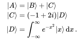
Note how the last line above involves infinitely many different kets, one for each real number x.

_

A Hilbert space is an abstract vector space possessing the structure of an inner product that allows length and angle to be measured. Furthermore, Hilbert spaces are complete: there are enough limits in the space to allow the techniques of calculus to be used.  Virtually all the quantum computing literature refers to a finite-dimensional complex vector space by the name ‘Hilbert space’, and we will use H to denote such a space. Hilbert spaces of interest for quantum computing will typically have dimension 2^n, for some positive integer n. This is because, as with classical information, we will construct larger state spaces by concatenating a string of smaller systems, usually of size two.

______

______

Linear algebra:

Linear Algebra is a continuous form of mathematics and is applied throughout science and engineering because it allows you to model natural phenomena and to compute them efficiently. Because it is a form of continuous and not discrete mathematics, a lot of computer scientists don’t have a lot of experience with it. Linear Algebra is also central to almost all areas of mathematics like geometry and functional analysis. Its concepts are a crucial prerequisite for understanding the theory behind Machine Learning, especially if you are working with Deep Learning Algorithms.

Linear algebra is about linear combinations. That is, using arithmetic on columns of numbers called vectors and arrays of numbers called matrices, to create new columns and arrays of numbers. Linear algebra is the study of lines and planes, vector spaces and mappings that are required for linear transforms.

It is a relatively young field of study, having initially been formalized in the 1800s in order to find unknowns in systems of linear equations. A linear equation is just a series of terms and mathematical operations where some terms are unknown; for example:

y = 4^ x + 1

Equations like this are linear in that they describe a line on a two-dimensional graph. The line comes from plugging in different values into the unknown x to find out what the equation or model does to the value of y.

We can line up a system of equations with the same form with two or more unknowns.

_

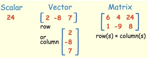
Linear algebra is a branch of mathematics, but the truth of it is that linear algebra is the mathematics of data. Matrices and vectors are the language of data. In Linear algebra, data is represented by linear equations, which are presented in the form of matrices and vectors. Therefore, you are mostly dealing with matrices and vectors rather than with scalars. When you have the right libraries, like Numpy, at your disposal, you can compute complex matrix multiplication very easily with just a few lines of code.

_

The application of linear algebra in computers is often called numerical linear algebra. It is more than just the implementation of linear algebra operations in code libraries; it also includes the careful handling of the problems of applied mathematics, such as working with the limited floating point precision of digital computers.

Computers are good at performing linear algebra calculations, and much of the dependence on Graphical Processing Units (GPUs) by modern machine learning methods such as deep learning because of their ability to compute linear algebra operations fast.

Efficient implementations of vector and matrix operations were originally implemented in the FORTRAN programming language in the 1970s and 1980s and a lot of code ported from those implementations, underlies much of the linear algebra performed using modern programming languages, such as Python.

Three popular open source numerical linear algebra libraries that implement these functions are:

Linear Algebra Package, or LAPACK.

Basic Linear Algebra Subprograms, or BLAS (a standard for linear algebra libraries).

Automatically Tuned Linear Algebra Software, or ATLAS.

Often, when you are calculating linear algebra operations directly or indirectly via higher-order algorithms, your code is very likely dipping down to use one of these, or similar linear algebra libraries. The name of one of more of these underlying libraries may be familiar to you if you have installed or compiled any of Python’s numerical libraries such as SciPy and NumPy.

_

Computational Rules:

1. Matrix-Scalar Operations

If you multiply, divide, subtract, or add a Scalar to a Matrix, you do so with every element of the Matrix.

2. Matrix-Vector Multiplication

Multiplying a Matrix by a Vector can be thought of as multiplying each row of the Matrix by the column of the Vector. The output will be a Vector that has the same number of rows as the Matrix.

3. Matrix-Matrix Addition and Subtraction

Matrix-Matrix Addition and Subtraction is fairly easy and straightforward. The requirement is that the matrices have the same dimensions and the result is a Matrix that has also the same dimensions. You just add or subtract each value of the first Matrix with its corresponding value in the second Matrix.

4. Matrix-Matrix Multiplication

Multiplying two Matrices together isn’t that hard either if you know how to multiply a Matrix by a Vector. Note that you can only multiply Matrices together if the number of the first Matrix’s columns matches the number of the second Matrix’s rows. The result will be a Matrix with the same number of rows as the first Matrix and the same number of columns as the second Matrix.

_

Until the 19th century, linear algebra was introduced through systems of linear equations and matrices. In modern mathematics, the presentation through vector spaces is generally preferred, since it is more synthetic, more general (not limited to the finite-dimensional case), and conceptually simpler, although more abstract. An element of a specific vector space may have various nature; for example, it could be a sequence, a function, a polynomial or a matrix. Linear algebra is concerned with those properties of such objects that are common to all vector spaces. Matrices allow explicit manipulation of finite-dimensional vector spaces and linear maps.

_

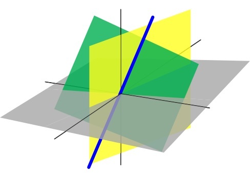
In the three-dimensional Euclidean space as seen in the figure above, these three planes represent solutions of linear equations and their intersection represents the set of common solutions: in this case, a unique point. The blue line is the common solution of a pair of linear equations.

_

Usage in quantum mechanics:

The mathematical structure of quantum mechanics is based in large part on linear algebra:

• Wave functions and other quantum states can be represented as vectors in a complex Hilbert space. (The exact structure of this Hilbert space depends on the situation.) In bra-ket notation, for example, an electron might be in “the state |ψ⟩ “. (Technically, the quantum states are rays of vectors in the Hilbert space, as c|ψ⟩ corresponds to the same state for any nonzero complex number c.)
• Quantum superpositions can be described as vector sums of the constituent states. For example, an electron in the state| 1⟩ + | 2 ⟩ is in a quantum superposition of the states| 1⟩ and | 2 ⟩.
• Measurements are associated with linear operators (called observables) on the Hilbert space of quantum states.
• Dynamics is also described by linear operators on the Hilbert space. For example, in the Schrödinger picture, there is a linear operator U with the property that if an electron is in state |ψ⟩ right now, then in one minute it will be in the state U|ψ⟩ , the same U for every possible |ψ⟩.
• Wave function normalization is scaling a wave function so that its norm is 1.

Since virtually every calculation in quantum mechanics involves vectors and linear operators, it can involve, and often does involve, bra-ket notation.

Quantum computation inherited linear algebra from quantum mechanics as the supporting language for describing this area. Therefore, it is essential to have a solid knowledge of the basic results of linear algebra to understand quantum computation and quantum algorithms.

_______

_______

Classical computing:

_

Theoretical computer science is essentially math, and subjects such as probability, statistics, linear algebra, graph theory, combinatorics and optimization are at the heart of artificial intelligence (AI), machine learning (ML), data science and computer science in general. Theoretical work in quantum computing requires expertise in quantum mechanics, linear algebra, theory of computation, information theory and information security.

_

Theory of computation:

In theoretical computer science and mathematics, the theory of computation is the branch that deals with how efficiently problems can be solved on a model of computation, using an algorithm. The field is divided into three major branches: automata theory and languages, computability theory, and computational complexity theory, which are linked by the question: “What are the fundamental capabilities and limitations of computers?”.

In order to perform a rigorous study of computation, computer scientists work with a mathematical abstraction of computers called a model of computation. There are several models in use, but the most commonly examined is the Turing machine. Computer scientists study the Turing machine because it is simple to formulate, can be analyzed and used to prove results, and because it represents what many consider the most powerful possible “reasonable” model of computation. It might seem that the potentially infinite memory capacity is an unrealizable attribute, but any decidable problem solved by a Turing machine will always require only a finite amount of memory. So in principle, any problem that can be solved (decided) by a Turing machine can be solved by a computer that has a finite amount of memory.

_

Now, let’s understand the basic terminologies, which are important and frequently used in Theory of Computation.

Symbol:

Symbol is the smallest building block, which can be any alphabet, letter or any picture.

A, b, c, 0, 1,…

Alphabets (Σ):

Alphabets are set of symbols, which are always finite.

Σ = {0,1} is an alphabet of binary digits.

Σ = {a, b, c}

Σ = {1, 2, 3, ….9} is an alphabet of decimal digits.

String:

String is a finite sequence of symbols from some alphabet. String is generally denoted as w and length of a string is denoted as |w|.

Empty string is the string with zero occurrence of symbols, represented as ε.

Number of Strings (of length 2) that can be generated over the alphabet {a, b}

a   a

a   b

b   a

b   b

Length of String |w| = 2

Number of Strings = 4

For alphabet {a, b} with length n, number of strings can be generated = 2ⁿ.

Note – If the number of ‘Σ’ is represented by |Σ|, then number of strings of length n, possible over Σ is |Σ|ⁿ.

Language:

A language is a set of strings, chosen from some Σ* or we can say- ‘A language is a subset of Σ* ‘. A language which can be formed over ‘ Σ ‘ can be Finite or Infinite.

Powers of ‘ Σ ‘ :
Say Σ = {a,b} then
Σ⁰ = Set of all strings over Σ of length 0. {ε}
Σ¹ = Set of all strings over Σ of length 1. {a, b}
Σ² = Set of all strings over Σ of length 2. {aa, ab, ba, bb}
i.e. |Σ²|= 4 and Similarly, |Σ³| = 8

Σ^* is a Universal Set.

Σ^* = Σ⁰ U Σ¹ U Σ² ………. = {ε} U {a, b} U {aa, ab, ba, bb} = ………….   //infinite language.

_

A computer is a physical device that helps us process information by executing algorithms. An algorithm is a well-defined procedure, with finite description, for realizing an information-processing task. An information-processing task can always be translated into a physical task. When designing complex algorithms and protocols for various information-processing tasks, it is very helpful, perhaps essential, to work with some idealized computing model. However, when studying the true limitations of a computing device, especially for some practical reason, it is important not to forget the relationship between computing and physics. Real computing devices are embodied in a larger and often richer physical reality than is represented by the idealized computing model. Quantum information processing is the result of using the physical reality that quantum theory tells us about for the purposes of performing tasks that were previously thought impossible or infeasible. Devices that perform quantum information processing are known as quantum computers.

_

Why should a person interested in quantum computation and quantum information spend time investigating classical computer science?

There are three good reasons for this effort.

First, classical computer science provides a vast body of concepts and techniques which may be reused to great effect in quantum computation and quantum information. Many of the triumphs of quantum computation and quantum information have come by combining existing ideas from computer science with novel ideas from quantum mechanics. For example, some of the fast algorithms for quantum computers are based upon the Fourier transform, a powerful tool utilized by many classical algorithms. Once it was realized that quantum computers could perform a type of Fourier transform much more quickly than classical computers this enabled the development of many important quantum algorithms.

Second, computer scientists have expended great effort understanding what resources are required to perform a given computational task on a classical computer. These results can be used as the basis for a comparison with quantum computation and quantum information. For example, much attention has been focused on the problem of finding the prime factors of a given number. On a classical computer this problem is believed to have no ‘efficient’ solution.  What is interesting is that an efficient solution to this problem is known for quantum computers. The lesson is that, for this task of finding prime factors, there appears to be a gap between what is possible on a classical computer and what is possible on a quantum computer. This is both intrinsically interesting, and also interesting in the broader sense that it suggests such a gap may exist for a wider class of computational problems than merely the finding of prime factors. By studying this specific problem further, it may be possible to discern features of the problem which make it more tractable on a quantum computer than on a classical computer, and then act on these insights to find interesting quantum algorithms for the solution of other problems.

Third, and most important, there is learning to think like a computer scientist. Computer scientists think in a rather different style than does a physicist or other natural scientist. Anybody wanting a deep understanding of quantum computation and quantum information must learn to think like a computer scientist at least some of the time; they must instinctively know what problems, what techniques, and most importantly what problems are of greatest interest to a computer scientist.

_

Conventional computers have two tricks that they do really well: they can store numbers in memory and they can process stored numbers with simple mathematical operations (like add and subtract). They can do more complex things by stringing together the simple operations into a series called an algorithm (multiplying can be done as a series of additions, for example). Both of a computer’s key tricks—storage and processing—are accomplished using switches called transistors, which are like microscopic versions of the switches you have on your wall for turning on and off the lights. A transistor can either be on or off, just as a light can either be lit or unlit. If it’s on, we can use a transistor to store a number one (1); if it’s off, it stores a number zero (0). Long strings of ones and zeros can be used to store any number, letter, or symbol using a code based on binary (so computers store an upper-case letter A as 1000001 and a lower-case one as 01100001). Each of the zeros or ones is called a binary digit (or bit) and, with a string of eight bits, you can store 255 different characters (such as A-Z, a-z, 0-9, and most common symbols). Computers calculate by using circuits called logic gates, which are made from a number of transistors connected together. Logic gates compare patterns of bits, stored in temporary memories called registers, and then turn them into new patterns of bits—and that’s the computer equivalent of what our human brains would call addition, subtraction, or multiplication. In physical terms, the algorithm that performs a particular calculation takes the form of an electronic circuit made from a number of logic gates, with the output from one gate feeding in as the input to the next.

_

The trouble with conventional computers is that they depend on conventional transistors. This might not sound like a problem if you go by the amazing progress made in electronics over the last few decades. When the transistor was invented, back in 1947, the switch it replaced (which was called the vacuum tube) was about as big as one of your thumbs. Now, a state-of-the-art microprocessor (single-chip computer) packs hundreds of millions (and up to 30 billion) transistors onto a chip of silicon the size of your fingernail! Chips like these, which are called integrated circuits, are an incredible feat of miniaturization. The high speed modern computer is fundamentally no different from its gargantuan 30 ton ancestors which were equipped with some 18000 vacuum tubes and 500 miles of wiring. Although computers have become more compact and considerably faster in performing their task, the task remains the same: to manipulate and interpret an encoding of binary bits into a useful computational result.

_

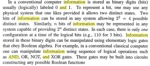
Classical computers, which we use on a daily basis, are built upon the concept of digital logic and bits. A bit is simply an idea, or an object, which can take on one of two distinct values, typically labelled 0 or 1. In computers this concept is usually embodied by transistors, which can be charged (1) or uncharged (0). A computer encodes information in a series of bits, and performs operations on them using circuits called logic gates. Logic gates simply apply a given rule to a bit. For example, an OR gate takes two bits as input, and outputs a single value. If either of the inputs is 1, the gate returns 1. Otherwise, it returns 0. Once the operations are finished, the information regarding the output can be decoded from the bits. Engineers can design circuits which perform addition and subtraction, multiplications… almost any operation that comes to mind, as long as the input and output information can be encoded in bits.

_

Classically, a compiler for a high-level programming language translates algebraic expressions into sequences of machine language instructions to evaluate the terms and operators in the expression.

Following instructions are supported on a classical computer:

1. Add
2. Subtract
3. Multiply
4. Divide

And with these most basic operations, there is ability to evaluate classical math functions:

1. Square root
2. Exponentials
3. Logarithms
4. Trigonometric functions
5. Statistical functions

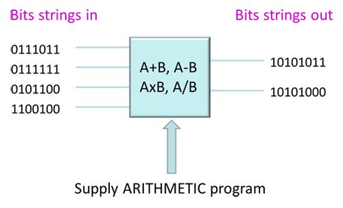
Classical computing is based in large part on modern mathematics and logic. We take modern digital computers and their ability to perform a multitude of different applications for granted. Our desktop PCs, laptops and smart phones can run spreadsheets, stream live video, allow us to chat with people on the other side of the world, and immerse us in realistic 3D environments. But at their core, all digital computers have something in common. They all perform simple arithmetic operations. Their power comes from the immense speed at which they are able to do this. Computers perform billions of operations per second. These operations are performed so quickly that they allow us to run very complex high level applications. Conventional digital computing can be summed up by the diagram shown in figure below.

Although there are many tasks that conventional computers are very good at, there are still some areas where calculations seem to be exceedingly difficult. Examples of these areas are: Image recognition, natural language (getting a computer to understand what we mean if we speak to it using our own language rather than a programming language), and tasks where a computer must learn from experience to become better at a particular task. Even though there has been much effort and research poured into this field over the past few decades, our progress in this area has been slow and the prototypes that we do have working usually require very large supercomputers to run them, consuming vast quantities of space and power.

_

Classical circuit:

Circuits are net-works composed of wires that carry bit values to gates that perform elementary operations on the bits. The circuits we consider will all be acyclic, meaning that the bits move through the circuit in a linear fashion, and the wires never feedback to a prior location in the circuit. A circuit Cn has n wires, and can be described by a circuit diagram shown in figure below for n=4. The input bits are written onto the wires entering the circuit from the left side of the diagram. The output bits are read-off the wires leaving the circuit at the right side of the diagram.

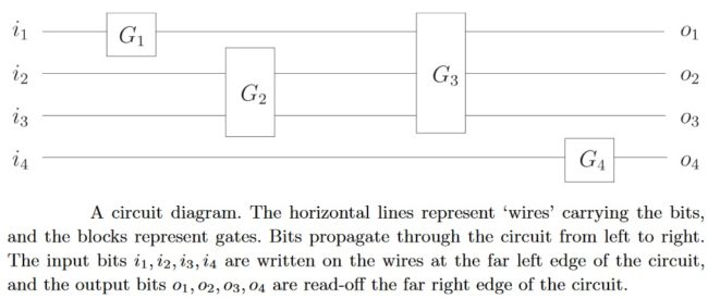
A circuit is an array or network of gates, which is the terminology often used in the quantum setting. The gates come from some finite family, and they take information from input wires and deliver information along some output wires.

An important notion is that of universality. It is convenient to show that a finite set of different gates is all we need to be able to construct a circuit for performing any computation we want.

_

A circuit is made up of wires and gates, which carry information around, and perform simple computational tasks, respectively. For example, figure below shows a simple circuit which takes as input a single bit, a. This bit is passed through a gate, which flips the bit, taking 1 to 0 and 0 to 1. The wires before and after the gate serve merely to carry the bit to and from the gate; they can represent movement of the bit through space, or perhaps just through time.

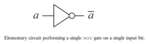
More generally, a circuit may involve many input and output bits, many wires, and many logical gates. A logic gate is a function f:{0,1}^k→{0,1}^l from some fixed number k of input bits to some fixed number l of output bits. For example, the gate is a gate with one input bit and one output bit which computes the function f(a)=1⊕a, where a is a single bit, and ⊕ is modulo 2 addition. It is also usual to make the convention that no loops are allowed in the circuit, to avoid possible instabilities. We say such a circuit is acyclic, and we adhere to the convention that circuits in the circuit model of computation be acyclic.

There are many other elementary logic gates which are useful for computation. A partial list includes the AND gate, the OR gate, the XOR gate, the NAND gate, and the NOR gate. Each of these gates takes two bits as input, and produces a single bit as output. The AND gate outputs 1 if and only if both of its inputs are 1. The OR gate outputs 1 if and only if at least one of its inputs is 1. The XOR gate outputs the sum, modulo 2, of its inputs. The NAND and NOR gates take the AND and, OR respectively, of their inputs, and then apply a NOT to whatever is output.

These simple circuit elements can be put together to perform an enormous variety of computations.

_

The most important characteristics of a computer is how fast it can perform calculations (the clock speed in our domestic PCs is a measure of this). This is determined by two main factors. One is the processor, which determined how many operations can be carried out on bits in a given time interval. The other is the nature of the calculation: how many operations on bits it takes to carry it out. This is why it is key to have optimized algorithms, you want to complete a given task in as few steps as possible. The problem is that even the most sophisticated versions of some tasks, like integer factoring, require an enormous amount of operations to be completed. These are the kind of tasks that could take billions of years to complete even on the best computers.

_

What we refer to as the universal computing machine was conceived by the man considered the father of computer sciences, Alan Turing, in 1936. Years before there were actual computers in the world, Turing suggested building a read-write head that would move a tape, read the different state in each frame, and replicate it according to commands it received. It sounds simplistic, but there is no fundamental difference between the theoretical Turing machine and laptop. The only difference is that laptop reads-writes so many frames per second that it’s impossible to discern that it’s actually calculating.  Classical computers perform these calculations by means of transistors. In 1947, William Shockley, Walter Brattain and John Bardeen built the first transistor – the word is an amalgam of “transfer” and “resistor.” The transistor is a kind of switch that sits within a slice of silicon and acts as the multi-state frame that Turing dreamed of. Turn on the switch and the electricity flows through the transistor; turn it off, and the electricity does not flow. Hence, the use of transistors in computers is binary: if the electricity flows through the transistor, the bit, or binary digit, is 1; and if the current does not flow, the bit is 0.

With transistors, the name of the game is miniaturization. The smaller the transistor, the more of them it is possible to compress into the silicon slice, and the more complex are the calculations one can perform. It took a whole decade to get from the one transistor to an integrated circuit of four transistors. Ten years later, in 1965, it had become possible to compress 64 transistors onto a chip. At this stage, Gordon Moore, who would go on to found Intel, predicted that the number of transistors per silicon slice would continue to grow exponentially. Moore’s Law states that every 2 years, like clockwork, engineers will succeed in miniaturizing and compressing double the number of transistors in an integrated circuit. Thus we got the golden age of computers: the Intel 286, with 134,000 transistors in 1982; the 386, with 275,000 transistors, in 1985; the 486, with 1,180,235 transistors, in 1989; and the Pentium, with 3.1 million transistors, in 1993. There was no reason to leave the house. Today, the human race is manufacturing dozens of billions of transistors per second. Your smartphone has about 2 to 4 billion transistors. According to a calculation made by the semiconductor analyst Jim Handy, since the first transistor was created in 1947, 2,913,276,327,576,980,000,000 transistors – that’s 2.9 sextillion – have been manufactured, and within a few years there will be more transistors in the world than all the cells in all the human bodies on earth.

_

The number of transistors per inch on integrated circuit will double every 2 years and this trend will continue for at least two decades. This prediction was formulated by Gordon Moore in 1965. Today, Moore’s Law still applies. If Moore’s Law is extrapolated naively to the future, it is learnt that sooner or later, each bit of information should be encoded by a physical system of subatomic size. If we’d continued to miniaturize transistors at the rate of Moore’s Law, we would have reached the stage of a transistor the size of an atom – and we would have had to split the atom. As a matter of fact, this point is substantiated by the survey made by Keyes in 1988 as shown in figure below. This plot shows the number of electrons required to store a single bit of information. An extrapolation of the plot suggests that we might be within the reach of atomic scale computations with in a decade or so at the atomic scale however.

_

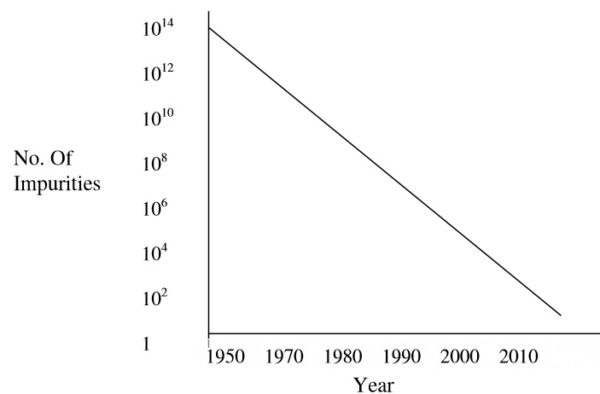
Figure above shows number of dopant impurities in logic in bipolar transistors with year.

_

The problem will arise when the new technologies allow to manufacture chips of around 5 nm.  Modern microprocessors are working on 64-bit architectures integrating more than 700 million transistors and they can operate at frequencies above 3 GHz. For instance, the third-generation Intel Core (2012) evolved from 32 nm wide to 22 nm, thus allowing duplication of the number of transistors per surface unit.  A dual-core mobile variant of the Intel Core i3/i5/i7 has around 1.75 billion transistors for a die size of 101.83 mm². This works out at a density of 17.185 million transistors per square millimetre. Moreover, a larger number of transistors means that a given computer system could be able to do more tasks rapidly. But, following the arguments of Feynman there is an “essential limit” for this to be done. The limits of the so-called “Tunnel Effect”

The fact is that increasingly smaller microchips are manufactured. And the smaller is the device, the faster the computing process is reached. However, we cannot infinitely diminish the size of the chips. There is a limit at which they stop working correctly. When it comes down to the nanometer size, electrons escape from the channels where they circulate through the so-called “tunnel effect”, a typically quantum phenomenon. Electrons are quantum particles and they have wave-like behavior, hence, there is a possibility that a part of such electrons can pass through the walls between which they are confined. Under these conditions the chip stops working properly. In this context the traditional digital computing should not be far from the limits, since we have already reached sizes of only a few tens of nanometers. But… where is the real limit?

The answer may have much to do with the world of the very small. In this respect, the various existing methods to estimate the size of the atomic radius give values between 0.5 and 5Å. The size of current transistor is of the order of nanometers (nm), while the size of typical atoms is of the order of angstroms (Å). But 10 Å = 1 nm. We only have to go one order of magnitude further, prior to designing our computers considering the restrictions imposed by quantum mechanics! Tiny matter obeys the rules of quantum mechanics, which are quite different from the classical rules that determine the properties of conventional logic gates.

_

The process of miniaturization that has made current classical computers so powerful and cheap, has already reached micro-levels where quantum effects occur. Chip-makers tend to go to great lengths to suppress those quantum effects, but instead one might also try to work with them, enabling further miniaturization. With the size of components in classical computers shrinking to where the behaviour of the components is practically dominated by quantum theory than classical theory, researchers have begun investigating the potential of these quantum behaviours for computation. Surprisingly it seems that a computer whose components are all to function in a quantum way are more powerful than any classical computer can be. It is the physical limitations of the classical computer and the possibilities for the quantum computer to perform certain useful tasks more rapidly than any classical computer, which drive the study of quantum computing.

_

Figure below shows Memory chip from a USB flash memory stick:

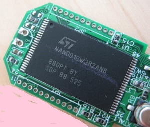
This memory chip from a typical USB stick contains an integrated circuit that can store 512 megabytes of data. That’s roughly 500 million characters (536,870,912 to be exact), each of which needs eight binary digits—so we’re talking about 4 billion (4,000 million) transistors in all (4,294,967,296 if you’re being picky) packed into an area the size of a postage stamp! It sounds amazing. The more information you need to store, the more binary ones and zeros—and transistors—you need to do it. Since most conventional computers can only do one thing at a time, the more complex the problem you want them to solve, the more steps they’ll need to take and the longer they’ll need to do it. Some computing problems are so complex that they need more computing power and time than any modern machine could reasonably supply; computer scientists call those intractable problems. As Moore’s Law advances, so the number of intractable problems diminishes: computers get more powerful and we can do more with them. The trouble is, transistors are just about as small as we can make them: we’re getting to the point where the laws of physics seem likely to put a stop to Moore’s Law. As a consequence of the relentless, Moore’s law-driven miniaturization of silicon devices, it is now possible to make transistors that are only few tens of atoms long. At this scale, however, quantum physics effects begin to prevent transistors from performing reliably – a phenomenon that limits prospects for future progress in conventional computing and end to Moore’s law.

Unfortunately, there are still hugely difficult computing problems we can’t tackle because even the most powerful computers find them intractable. That’s one of the reasons why people are now getting interested in quantum computing.

_____

_____

Quantum mechanics:

Quantum mechanics is the science of the very small. It explains the behavior of matter and its interactions with energy on the scale of atoms and subatomic particles. By contrast, classical physics explains matter and energy only on a scale familiar to human experience, including the behavior of astronomical bodies such as the Moon. Classical physics is still used in much of modern science and technology. However, towards the end of the 19th century, scientists discovered phenomena in both the large (macro) and the small (micro) worlds that classical physics could not explain. The desire to resolve inconsistencies between observed phenomena and classical theory led to two major revolutions in physics that created a shift in the original scientific paradigm: the theory of relativity and the development of quantum mechanics.

_

Newtonian physics thought of the world as composed of distinct objects, much like tennis balls or stone blocks. In this model, the universe is a giant machine of interlocking parts in which every action produces an equal and opposite reaction. Unfortunately the Newtonian world breaks down at the subatomic level. In the quantum world, everything seems to be an ocean of interconnected possibilities. Every particle is just a wave function and could be anywhere at anytime; it could even be at several places simultaneously. Swirling electrons occupy two positions at once, and possess dual natures — they can be both waves and particles simultaneously. In recent times, physicists have discovered a phenomenon called quantum entanglement. In an entangled system, two seemingly separate particles can behave as an inseparable whole. Theoretically, if one separates the two entangled particles, one would find that their velocity of spin would be identical but in opposite directions. They are quantum twins. Despite the seeming irrationality of these concepts, scientists over the last 120 years have demonstrated that this realm — known as quantum mechanics — is the foundation on which our physical existence is built. It is one of the most successful theories in modern science. Without it, we would not have such marvels as atomic clocks, computers, lasers, LEDs, global positioning systems and magnetic resonance imaging, among many other innovations.

_

Prior to the emergence of quantum mechanics, fundamental physics was marked by a peculiar dualism. On the one hand, we had electric and magnetic fields, governed by Maxwell’s equations. The fields filled all of space and were continuous. On the other hand, we had atoms, governed by Newtonian mechanics. The atoms were spatially limited — indeed, quite small — discrete objects. At the heart of this dualism was the contrast of light and substance, a theme that has fascinated not only scientists but artists and mystics for many centuries. One of the glories of quantum theory is that it has replaced that dualistic view of matter with a unified one. We learned to make fields from photons, and atoms from electrons (together with other elementary particles). Both photons and electrons are described using the same mathematical structure. They are particles, in the sense that they come in discrete units with definite, reproducible properties. But the new quantum-mechanical sort of “particle” cannot be associated with a definite location in space. Instead, the possible results of measuring its position are given by a probability distribution. And that distribution is given as the square of a space-filling field, its so-called wave function.

_

Quantum mechanics (also known as quantum physics, quantum theory, the wave mechanical model, or matrix mechanics), including quantum field theory, is a fundamental theory in physics which describes nature at the smallest – including atomic and subatomic – scales.

Quantum theory’s development began in 1900 with a presentation by Max Planck to the German Physical Society, in which he introduced the idea that energy exists in individual units (which he called “quanta”), as does matter. Further developments by a number of scientists over the following thirty years led to the modern understanding of quantum theory.

The Essential Elements of Quantum Theory:

1. Energy, like matter, consists of discrete units, rather than solely as a continuous wave.
2. Elementary particles of both energy and matter, depending on the conditions, may behave like either particles or waves.
3. The movement of elementary particles is inherently random, and, thus, unpredictable.
4. The simultaneous measurement of two complementary values, such as the position and momentum of an elementary particle, is inescapably flawed; the more precisely one value is measured, the more flawed will be the measurement of the other value.

Further Developments of Quantum Theory:

Niels Bohr proposed the Copenhagen interpretation of quantum theory, which asserts that a particle is whatever it is measured to be (for example, a wave or a particle) but that it cannot be assumed to have specific properties, or even to exist, until it is measured. In short, Bohr was saying that objective reality does not exist. This translates to a principle called superposition that claims that while we do not know what the state of any object is, it is actually in all possible states simultaneously, as long as we don’t look to check.

The second interpretation of quantum theory is the multiverse or many-worlds theory. It holds that as soon as a potential exists for any object to be in any state, the universe of that object transmutes into a series of parallel universes equal to the number of possible states in which that the object can exist, with each universe containing a unique single possible state of that object. Furthermore, there is a mechanism for interaction between these universes that somehow permits all states to be accessible in some way and for all possible states to be affected in some manner. Stephen Hawking and the late Richard Feynman are among the scientists who have expressed a preference for the many-worlds theory.

_

Classical physics, the description of physics existing before the formulation of the theory of relativity and of quantum mechanics, describes nature at ordinary (macroscopic) scale. Most theories in classical physics can be derived from quantum mechanics as an approximation valid at large (macroscopic) scale. Quantum mechanics differs from classical physics in that energy, momentum, angular momentum, and other quantities of a bound system are restricted to discrete values (quantization), objects have characteristics of both particles and waves (wave-particle duality), and there are limits to how accurately the value of a physical quantity can be predicted prior to its measurement, given a complete set of initial conditions (the uncertainty principle).

_

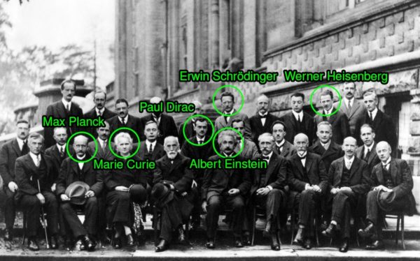
Quantum mechanics gradually arose from theories to explain observations which could not be reconciled with classical physics, such as Max Planck’s solution in 1900 to the black-body radiation problem, and from the correspondence between energy and frequency in Albert Einstein’s 1905 paper which explained the photoelectric effect. Early quantum theory was profoundly re-conceived in the mid-1920s by Erwin Schrödinger, Werner Heisenberg, Max Born and others. The modern theory is formulated in various specially developed mathematical formalisms. In one of them, a mathematical function, the wave function, provides information about the probability amplitude of energy, momentum, and other physical properties of a particle.

_

Many aspects of quantum mechanics are counterintuitive and can seem paradoxical because they describe behavior quite different from that seen at larger scales.

For example, the uncertainty principle of quantum mechanics means that the more closely one pins down one measurement (such as the position of a particle), the less accurate another complementary measurement pertaining to the same particle (such as its speed) must become.

Another example is entanglement, in which a measurement of any two-valued state of a particle (such as light polarized up or down) made on either of two “entangled” particles that are very far apart causes a subsequent measurement on the other particle to always be the other of the two values (such as polarized in the opposite direction).

A final example is superfluidity, in which a container of liquid helium, cooled down to near absolute zero in temperature spontaneously flows (slowly) up and over the opening of its container, against the force of gravity.

_

The building blocks of quantum mechanics:

The birth of quantum mechanics took place the first 27 years of the twentieth century to overcome the severe limitations in the validity of classical physics, with the first inconsistency being the Plank’s radiation law. Einstein, Debye, Bohr, de Broglie, Compton, Heisenberg, Schrödinger, Dirac amongst others were the pioneers in developing the theory of quantum mechanics as we know it today.

The fundamental building blocks of quantum mechanics are:

1. Quantisation: energy, momentum, angular momentum and other physical quantities of a bound system are restricted to discrete values (quantised)
2. Wave-particle duality: objects are both waves and particles
3. Heisenberg principle: the more precise the position of some particle is determined, the less precise its momentum can be known, and vice versa. Thus there is a fundamental limit to the measurement precision of physical quantities of a particle
4. Superposition: two quantum states can be added together, and the result is another valid quantum state
5. Entanglement: when the quantum state of any particle belonging to a system cannot be described independently of the state of the other particles, even when separated by a large distance, the particles are entangled
6. Fragility: by measuring a quantum system we destroy any previous information. From this, it follows the no-cloning theorem that states: it is impossible to create an identical copy of an arbitrary unknown quantum state

_

To understand how things work in the real world, quantum mechanics must be combined with other elements of physics – principally, Albert Einstein’s special theory of relativity, which explains what happens when things move very fast – to create what are known as quantum field theories. Three different quantum field theories deal with three of the four fundamental forces by which matter interacts: electromagnetism, which explains how atoms hold together; the strong nuclear force, which explains the stability of the nucleus at the heart of the atom; and the weak nuclear force, which explains why some atoms undergo radioactive decay.

_

Copenhagen interpretation:

Bohr, Heisenberg, and others tried to explain what these experimental results and mathematical models really mean. Their description, known as the Copenhagen interpretation of quantum mechanics, aimed to describe the nature of reality that was being probed by the measurements and described by the mathematical formulations of quantum mechanics.

The main principles of the Copenhagen interpretation are:

1. A system is completely described by a wave function, usually represented by the Greek letter ψ (“psi”). (Heisenberg)
2. How ψ changes over time is given by the Schrödinger equation.
3. The description of nature is essentially probabilistic. The probability of an event—for example, where on the screen a particle shows up in the double-slit experiment—is related to the square of the absolute value of the amplitude of its wave function. (Born rule, due to Max Born, which gives a physical meaning to the wave function in the Copenhagen interpretation: the probability amplitude)
4. It is not possible to know the values of all of the properties of the system at the same time; those properties that are not known with precision must be described by probabilities. (Heisenberg’s uncertainty principle)
5. Matter, like energy, exhibits a wave–particle duality. An experiment can demonstrate the particle-like properties of matter, or its wave-like properties; but not both at the same time. (Complementarity principle due to Bohr)
6. Measuring devices are essentially classical devices, and measure classical properties such as position and momentum.
7. The quantum mechanical description of large systems should closely approximate the classical description. (Correspondence principle of Bohr and Heisenberg)

_

Uncertainty principle:

Suppose it is desired to measure the position and speed of an object—for example a car going through a radar speed trap. It can be assumed that the car has a definite position and speed at a particular moment in time. How accurately these values can be measured depends on the quality of the measuring equipment. If the precision of the measuring equipment is improved, it provides a result closer to the true value. It might be assumed that the speed of the car and its position could be operationally defined and measured simultaneously, as precisely as might be desired.

In 1927, Heisenberg proved that this last assumption is not correct. Quantum mechanics shows that certain pairs of physical properties, for example position and speed, cannot be simultaneously measured, nor defined in operational terms, to arbitrary precision: the more precisely one property is measured, or defined in operational terms, the less precisely can the other. This statement is known as the uncertainty principle. The uncertainty principle is not only a statement about the accuracy of our measuring equipment, but, more deeply, is about the conceptual nature of the measured quantities—the assumption that the car had simultaneously defined position and speed does not work in quantum mechanics. On a scale of cars and people, these uncertainties are negligible, but when dealing with atoms and electrons they become critical.

Heisenberg gave, as an illustration, the measurement of the position and momentum of an electron using a photon of light. In measuring the electron’s position, the higher the frequency of the photon, the more accurate is the measurement of the position of the impact of the photon with the electron, but the greater is the disturbance of the electron. This is because from the impact with the photon, the electron absorbs a random amount of energy, rendering the measurement obtained of its momentum increasingly uncertain (momentum is velocity multiplied by mass), for one is necessarily measuring its post-impact disturbed momentum from the collision products and not its original momentum. With a photon of lower frequency, the disturbance (and hence uncertainty) in the momentum is less, but so is the accuracy of the measurement of the position of the impact.

At the heart of the uncertainty principle is not a mystery, but the simple fact that for any mathematical analysis in the position and velocity domains (Fourier analysis), achieving a sharper (more precise) curve in the position domain can only be done at the expense of a more gradual (less precise) curve in the speed domain, and vice versa. More sharpness in the position domain requires contributions from more frequencies in the speed domain to create the narrower curve, and vice versa. It is a fundamental tradeoff inherent in any such related or complementary measurements, but is only really noticeable at the smallest (Planck) scale, near the size of elementary particles.

The uncertainty principle shows mathematically that the product of the uncertainty in the position and momentum of a particle (momentum is velocity multiplied by mass) could never be less than a certain value, and that this value is related to Planck’s constant.

_

Wave function collapse:

Wave function collapse means that a measurement has forced or converted a quantum (probabilistic) state into a definite measured value. This phenomenon is only seen in quantum mechanics rather than classical mechanics. For example, before a photon actually “shows up” on a detection screen it can be described only with a set of probabilities for where it might show up. When it does appear, for instance in the CCD of an electronic camera, the time and the space where it interacted with the device are known within very tight limits. However, the photon has disappeared in the process of being captured (measured), and its quantum wave function has disappeared with it. In its place some macroscopic physical change in the detection screen has appeared, e.g., an exposed spot in a sheet of photographic film, or a change in electric potential in some cell of a CCD.

_

Eigenstates and eigenvalues:

Because of the uncertainty principle, statements about both the position and momentum of particles can only assign a probability that the position or momentum will have some numerical value. The uncertainty principle also says that eliminating uncertainty about position maximises uncertainty about momentum, and eliminating uncertainty about momentum maximizes uncertainty about position. A probability distribution assigns probabilities to all possible values of position and momentum. Schrödinger’s wave equation gives wavefunction solutions, the squares of which are probabilities of where the electron might be, just as Heisenberg’s probability distribution does.

In the everyday world, it is natural and intuitive to think of every object being in its own eigenstate. This is another way of saying that every object appears to have a definite position, a definite momentum, a definite measured value, and a definite time of occurrence. However, the uncertainty principle says that it is impossible to measure the exact value for the momentum of a particle like an electron, given that its position has been determined at a given instant. Likewise, it is impossible to determine the exact location of that particle once its momentum has been measured at a particular instant.

Therefore, it became necessary to formulate clearly the difference between the state of something that is uncertain in the way just described, such as an electron in a probability cloud, and the state of something having a definite value. When an object can definitely be “pinned down” in some respect, it is said to possess an eigenstate. As stated above, when the wavefunction collapses because the position of an electron has been determined, the electron’s state becomes an “eigenstate of position”, meaning that its position has a known value, an eigenvalue of the eigenstate of position.

The word “eigenstate” is derived from the German/Dutch word “eigen”, meaning “inherent” or “characteristic”. An eigenstate is the measured state of some object possessing quantifiable characteristics such as position, momentum, etc. The state being measured and described must be observable (i.e. something such as position or momentum that can be experimentally measured either directly or indirectly), and must have a definite value, called an eigenvalue.

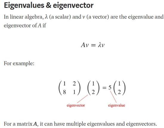
Eigenvalue also refers to a mathematical property of square matrices, a usage pioneered by the mathematician David Hilbert in 1904. Some such matrices are called self-adjoint operators, and represent observables in quantum mechanics as seen in the figure below:

_

The Pauli exclusion principle:

In 1924, Wolfgang Pauli proposed a new quantum degree of freedom (or quantum number), with two possible values, to resolve inconsistencies between observed molecular spectra and the predictions of quantum mechanics. In particular, the spectrum of atomic hydrogen had a doublet, or pair of lines differing by a small amount, where only one line was expected. Pauli formulated his exclusion principle, stating, “There cannot exist an atom in such a quantum state that two electrons within [it] have the same set of quantum numbers.” A year later, Uhlenbeck and Goudsmit identified Pauli’s new degree of freedom with the property called spin whose effects were observed in the Stern–Gerlach experiment.

_

Dirac wave equation:

In 1928, Paul Dirac extended the Pauli equation, which described spinning electrons, to account for special relativity. The result was a theory that dealt properly with events, such as the speed at which an electron orbits the nucleus, occurring at a substantial fraction of the speed of light. By using the simplest electromagnetic interaction, Dirac was able to predict the value of the magnetic moment associated with the electron’s spin, and found the experimentally observed value, which was too large to be that of a spinning charged sphere governed by classical physics. He was able to solve for the spectral lines of the hydrogen atom, and to reproduce from physical first principles Sommerfeld’s successful formula for the fine structure of the hydrogen spectrum. Dirac’s equations sometimes yielded a negative value for energy, for which he proposed a novel solution: he posited the existence of an antielectron and of a dynamical vacuum. This led to the many-particle quantum field theory.

_

Two-state quantum system:

In quantum mechanics, a two-state system (also known as a two-level system) is a quantum system that can exist in any quantum superposition of two independent (physically distinguishable) quantum states. The Hilbert space describing such a system is two-dimensional. Therefore, a complete basis spanning the space will consist of two independent states. Any two-state system can also be seen as a qubit. In quantum computing, a qubit or quantum bit is the basic unit of quantum information—the quantum version of the classical binary bit physically realized with a two-state device. A qubit is a two-state (or two-level) quantum-mechanical system, one of the simplest quantum systems displaying the peculiarity of quantum mechanics. Examples include: the spin of the electron in which the two levels can be taken as spin up and spin down; or the polarization of a single photon in which the two states can be taken to be the vertical polarization and the horizontal polarization. In a classical system, a bit would have to be in one state or the other. However, quantum mechanics allows the qubit to be in a coherent superposition of both states simultaneously, a property which is fundamental to quantum mechanics and quantum computing.

Two-state systems are the simplest quantum systems that can exist, since the dynamics of a one-state system is trivial (i.e. there is no other state the system can exist in). The mathematical framework required for the analysis of two-state systems is that of linear differential equations and linear algebra of two-dimensional spaces. As a result, the dynamics of a two-state system can be solved analytically without any approximation. The generic behavior of the system is that the wavefunction’s amplitude oscillates between the two states.

_

Quantum entanglement:

The Pauli exclusion principle says that two electrons in one system cannot be in the same state. Nature leaves open the possibility, however, that two electrons can have both states “superimposed” over each of them. Nothing is certain until the superimposed waveforms “collapse”. At that instant an electron shows up somewhere in accordance with the probability that is the square of the absolute value of the sum of the complex-valued amplitudes of the two superimposed waveforms. The situation there is already very abstract.  A concrete way of thinking about entangled photons, photons in which two contrary states are superimposed on each of them in the same event, is as follows:

Imagine that we have two color-coded states of photons: one state labeled blue and another state labeled red. Let the combination of the red and the blue state appear (in imagination) as a purple state. We consider a case in which two photons are produced as the result of one single atomic event. Perhaps they are produced by the excitation of a crystal that characteristically absorbs a photon of a certain frequency and emits two photons of half the original frequency. In this case, the photons are connected with each other via their shared origin in a single atomic event. This setup results in combined states of the photons. So the two photons come out purple. If the experimenter now performs some experiment that determines whether one of the photons is either blue or red, then that experiment changes the photon involved from one having a combination of blue and red characteristics to a photon that has only one of those characteristics. The problem that Einstein had with such an imagined situation was that if one of these photons had been kept bouncing between mirrors in a laboratory on earth, and the other one had traveled halfway to the nearest star, when its twin was made to reveal itself as either blue or red, that meant that the distant photon now had to lose its purple status too. So whenever it might be investigated after its twin had been measured, it would necessarily show up in the opposite state to whatever its twin had revealed.

In trying to show that quantum mechanics was not a complete theory, Einstein started with the theory’s prediction that two or more particles that have interacted in the past can appear strongly correlated when their various properties are later measured. He sought to explain this seeming interaction in a classical way, through their common past, and preferably not by some “spooky action at a distance”. The argument is worked out in a famous paper, Einstein, Podolsky, and Rosen (1935; abbreviated EPR), setting out what is now called the EPR paradox. Assuming what is now usually called local realism, EPR attempted to show from quantum theory that a particle has both position and momentum simultaneously, while according to the Copenhagen interpretation, only one of those two properties actually exists and only at the moment that it is being measured. EPR concluded that quantum theory is incomplete in that it refuses to consider physical properties that objectively exist in nature. (Einstein, Podolsky, & Rosen 1935 is currently Einstein’s most cited publication in physics journals.) In the same year, Erwin Schrödinger used the word “entanglement” and declared: “I would not call that one but rather the characteristic trait of quantum mechanics.” Ever since Irish physicist John Stewart Bell theoretically and experimentally disproved the “hidden variables” theory of Einstein, Podolsky, and Rosen, most physicists have accepted entanglement as a real phenomenon. However, there is some minority dispute. The Bell inequalities are the most powerful challenge to Einstein’s claims.

_

It is in the domain of information technology, however, that we might end up owing quantum mechanics our greatest debt. Researchers hope to use quantum principles to create an ultra-powerful computer that would solve problems that conventional computers cannot — from improving cybersecurity and modeling chemical reactions to formulating new drugs and making supply chains more efficient. This goal could revolutionize certain aspects of computing and open up a new world of technological possibilities. Thanks to advances at universities and industry research centers, a handful of companies have now rolled out prototype quantum computers, but the field is still wide open on fundamental questions about the hardware, software and connections necessary for quantum technologies to fulfil their potential.

______

Classical to Quantum Computation:

Computing has revolutionized information processing and management. As far back as Charles Babbage, it was recognized that information could be processed with physical systems, and more recently (e.g. the work of Rolf Landauer) that information must be represented in physical form and is thus subject to physical laws. The physical laws relevant to the information processing system are important to understanding the limitations of computation. Traditional computing devices adhere to the laws of classical mechanics and are thus referred to as “classical computers.” Proposed “quantum computers” are governed by the laws of quantum mechanics, leading to a dramatic difference in the computational capacity.

Fundamentally, Quantum Mechanics adds features that are absent in classical mechanics. To begin, physical quantities are “quantized,” i.e. cannot be subdivided. For example, light is quantized: the fundamental quantum of light is called the photon and cannot be subdivided into two photons. Quantum mechanics further requires physical states to evolve in such a way that cloning an arbitrary, unknown state into an independent copy is not possible. This is used in quantum cryptography to prevent information copying. Furthermore, quantum mechanics describes systems in terms of superpositions that allow multiple distinguishable inputs to be processed simultaneously, though only one can be observed at the end of processing, and the outcome is generally probabilistic in nature. Finally, quantum mechanics allows for correlations that are not possible to obtain in classical physics. Such correlations include what is called entanglement.

_

_

Classical machines couldn’t necessarily do all these computations efficiently, though. Let’s say you wanted to understand something like the chemical behavior of a molecule. This behavior depends on the behavior of the electrons in the molecule, which exist in a superposition of many classical states. Making things messier, the quantum state of each electron depends on the states of all the others — due to the quantum-mechanical phenomenon known as entanglement. Classically calculating these entangled states in even very simple molecules can become a nightmare of exponentially increasing complexity.

In order to describe a simple molecule with 300 atoms – penicillin, let’s say – we will need 2 to the 300th power classic transistors – which is more than the number of atoms in the universe. And that is only to describe the molecule at a particular moment. To run it in a simulation would require us to build another few universes to supply all the material needed.

A quantum computer, by contrast, can deal with the intertwined fates of the electrons under study by superposing and entangling its own quantum bits. This enables the computer to process extraordinary amounts of information. Each single qubit you add doubles the states the system can simultaneously store: Two qubits can store four states, three qubits can store eight states, and so on. Thus, you might need just 50 entangled qubits to model quantum states that would require exponentially many classical bits — 1.125 quadrillion to be exact — to encode. A quantum machine could therefore make the classically intractable problem of simulating large quantum-mechanical systems tractable, or so it appeared. “Nature isn’t classical, dammit, and if you want to make a simulation of nature, you’d better make it quantum mechanical,” the physicist Richard Feynman famously quipped in 1981. “And by golly it’s a wonderful problem, because it doesn’t look so easy.”

_

Classical computing relies, at its ultimate level, on principles expressed by Boolean algebra, operating with a (usually) 7-mode logic gate principle, though it is possible to exist with only three modes (which are AND, NOT, and COPY). Data must be processed in an exclusive binary state at any point in time – that is, either 0 (off / false) or 1 (on / true). These values are binary digits, or bits. The millions of transistors at the heart of computers can only be in one state at any point. While the time that each transistor need be either in 0 or 1 before switching states is now measurable in billionths of a second, there is still a limit as to how quickly these devices can be made to switch state. As we progress to smaller and faster circuits, we begin to reach the physical limits of materials and the threshold for classical laws of physics to apply. Beyond this, the quantum world takes over, which opens a potential as great as the challenges that are presented.

The Quantum computer, by contrast, can work with a two-mode logic gate: XOR and a mode we’ll call QO1 (the ability to change 0 into a superposition of 0 and 1, a logic gate which cannot exist in classical computing). In a quantum computer, a number of elemental particles such as electrons or photons can be used (in practice, success has also been achieved with ions), with either their charge or polarization acting as a representation of 0 and/or 1. Each of these particles is known as a quantum bit, or qubit, the nature and behavior of these particles form the basis of quantum computing. The two most relevant aspects of quantum physics are the principles of superposition and entanglement.

Think of a qubit as an electron in a magnetic field. The electron’s spin may be either in alignment with the field, which is known as a spin-up state, or opposite to the field, which is known as a spin-down state. Changing the electron’s spin from one state to another is achieved by using a pulse of energy, such as from a laser – let’s say that we use 1 unit of laser energy. But what if we only use half a unit of laser energy and completely isolate the particle from all external influences? According to quantum law, the particle then enters a superposition of states, in which it behaves as if it were in both states simultaneously. Each qubit utilized could take a superposition of both 0 and 1.

Entanglement Particles (such as photons, electrons, or qubits) that have interacted at some point retain a type of connection and can be entangled with each other in pairs, in a process known as correlation. Knowing the spin state of one entangled particle – up or down – allows one to know that the spin of its mate is in the opposite direction. Even more amazing is the knowledge that, due to the phenomenon of superposition, the measured particle has no single spin direction before being measured, but is simultaneously in both a spin-up and spin-down state. The spin state of the particle being measured is decided at the time of measurement and communicated to the correlated particle, which simultaneously assumes the opposite spin direction to that of the measured particle. This is a real phenomenon (Einstein called it “spooky action at a distance”), the mechanism of which cannot, as yet, be explained by any theory – it simply must be taken as given. Quantum entanglement allows qubits that are separated by incredible distances to interact with each other instantaneously (not limited to the speed of light). No matter how great the distance between the correlated particles, they will remain entangled as long as they are isolated.

Taken together, quantum superposition and entanglement create an enormously enhanced computing power. Where a 2-bit register in an ordinary computer can store only one of four binary configurations (00, 01, 10, or 11) at any given time, a 2-qubit register in a quantum computer can store all four numbers simultaneously, because each qubit represents two values. If more qubits are added, the increased capacity is expanded exponentially.

Quantum Programming:

Perhaps even more intriguing than the sheer power of quantum computing is the ability that it offers to write programs in a completely new way. For example, a quantum computer could incorporate a programming sequence that would be along the lines of “take all the superpositions of all the prior computations” – something which is meaningless with a classical computer – which would permit extremely fast ways of solving certain mathematical problems, such as factorization of large numbers.

There have been two notable successes thus far with quantum programming. The first occurred in 1994 by Peter Shor who developed a quantum algorithm that could efficiently factorize large numbers. It centers on a system that uses number theory to estimate the periodicity of a large number sequence. The other major breakthrough happened with Lov Grover in1996, with a very fast algorithm that is proven to be the fastest possible for searching through unstructured databases. The algorithm is so efficient that it requires only, on average, roughly N square root (where N is the total number of elements) searches to find the desired result, as opposed to a search in classical computing, which on average needs N searches.

______

______

History of quantum computing:

_

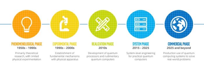
As early as 1959 the American physicist and Nobel laureate Richard Feynman noted that, as electronic components begin to reach microscopic scales, effects predicted by quantum mechanics occur—which, he suggested, might be exploited in the design of more powerful computers. In particular, quantum researchers hope to harness a phenomenon known as superposition. In the quantum mechanical world, objects do not necessarily have clearly defined states, as demonstrated by the famous experiment in which a single photon of light passing through a screen with two small slits will produce a wavelike interference pattern, or superposition of all available paths. However, when one slit is closed—or a detector is used to determine which slit the photon passed through—the interference pattern disappears. In consequence, a quantum system “exists” in all possible states before a measurement “collapses” the system into one state. Harnessing this phenomenon in a computer promises to expand computational power greatly. A traditional digital computer employs binary digits, or bits, that can be in one of two states, represented as 0 and 1; thus, for example, a 4-bit computer register can hold any one of 16 (2⁴) possible numbers. In contrast, a quantum bit (qubit) exists in a wavelike superposition of values from 0 to 1; thus, for example, a 4-qubit computer register can hold 16 different numbers simultaneously. In theory, a quantum computer can therefore operate on a great many values in parallel, so that a 30-qubit quantum computer would be comparable to a digital computer capable of performing 10 trillion floating-point operations per second (TFLOPS)—comparable to the speed of the fastest supercomputers.

During the 1980s and ’90s the theory of quantum computers advanced considerably beyond Feynman’s early speculations. In 1985 David Deutsch of the University of Oxford described the construction of quantum logic gates for a universal quantum computer, and in 1994 Peter Shor of AT&T devised an algorithm to factor numbers with a quantum computer that would require as few as six qubits (although many more qubits would be necessary for factoring large numbers in a reasonable time). When a practical quantum computer is built, it will break current encryption schemes based on multiplying two large primes; in compensation, quantum mechanical effects offer a new method of secure communication known as quantum encryption. However, actually building a useful quantum computer has proved difficult. Although the potential of quantum computers is enormous, the requirements are equally stringent. A quantum computer must maintain coherence between its qubits (known as quantum entanglement) long enough to perform an algorithm; because of nearly inevitable interactions with the environment (decoherence), practical methods of detecting and correcting errors need to be devised; and, finally, since measuring a quantum system disturbs its state, reliable methods of extracting information must be developed. Plans for building quantum computers have been proposed; although several demonstrate the fundamental principles, none is beyond the experimental stage.

In 1998 Isaac Chuang of the Los Alamos National Laboratory, Neil Gershenfeld of the Massachusetts Institute of Technology (MIT), and Mark Kubinec of the University of California at Berkeley created the first quantum computer (2-qubit) that could be loaded with data and output a solution. Although their system was coherent for only a few nanoseconds and trivial from the perspective of solving meaningful problems, it demonstrated the principles of quantum computation. Rather than trying to isolate a few subatomic particles, they dissolved a large number of chloroform molecules (CHCL3) in water at room temperature and applied a magnetic field to orient the spins of the carbon and hydrogen nuclei in the chloroform. (Because ordinary carbon has no magnetic spin, their solution used an isotope, carbon-13.) A spin parallel to the external magnetic field could then be interpreted as a 1 and an antiparallel spin as 0, and the hydrogen nuclei and carbon-13 nuclei could be treated collectively as a 2-qubit system. In addition to the external magnetic field, radio frequency pulses were applied to cause spin states to “flip,” thereby creating superimposed parallel and antiparallel states. Further pulses were applied to execute a simple algorithm and to examine the system’s final state. This type of quantum computer can be extended by using molecules with more individually addressable nuclei. In fact, in March 2000 Emanuel Knill, Raymond Laflamme, and Rudy Martinez of Los Alamos and Ching-Hua Tseng of MIT announced that they had created a 7-qubit quantum computer using trans-crotonic acid. However, many researchers are skeptical about extending magnetic techniques much beyond 10 to 15 qubits because of diminishing coherence among the nuclei. Just one week before the announcement of a 7-qubit quantum computer, physicist David Wineland and colleagues at the U.S. National Institute for Standards and Technology (NIST) announced that they had created a 4-qubit quantum computer by entangling four ionized beryllium atoms using an electromagnetic “trap.” After confining the ions in a linear arrangement, a laser cooled the particles almost to absolute zero and synchronized their spin states. Finally, a laser was used to entangle the particles, creating a superposition of both spin-up and spin-down states simultaneously for all four ions. Again, this approach demonstrated basic principles of quantum computing, but scaling up the technique to practical dimensions remains problematic.

_

1994

Shor’s Factoring Algorithm

MIT’s Peter Shor shows that it’s possible to factor a number into its primes efficiently on a quantum computer — a problem that takes classical computers “an exponentially long time” to solve for large numbers. His algorithm launches an explosion of theoretical and experimental interest in the field of quantum computing.

1995

Quantum Error Correction

Quantum error correction emerges from several groups around the world, including IBM. The theory shows that it’s possible to use a subtle redundancy to protect against environmental noise, making the physical realization of quantum computing significantly more tenable.

1996

DiVincenzo Criteria

IBM researcher David DiVincenzo outlines five minimal requirements for creating a quantum computer: (1) a well-defined scalable qubit array; (2) an ability to initialize the state of the qubits to a simple fiducial state; (3) a “universal” set of quantum gates; (4) long coherence times, much longer than the gate-operation time; (5) single-qubit measurement.

1997

Topological Codes

The first topological quantum error correcting code, known as the surface code, is proposed by California Institute of Technology professor Alexei Kitaev. The surface code is currently considered the most promising platform for realizing a scalable, fault-tolerant quantum computer.

2001

Experimentally Factoring

Shor’s algorithm is demonstrated for the first time in a real quantum computing experiment, albeit with a very pedestrian problem: 15=3×5. The IBM system employed qubits in nuclear spins, similar to an MRI machine.

2004

Circuit QED

Robert Schoelkopf and his collaborators at Yale University invent circuit QED, a means of studying the interaction of a photon and an artificial quantum object on a chip. Their work established the standard for coupling and reading out superconducting qubits as systems continue to scale.

2007

Transmon Superconducting Qubit

Schoelkopf and his collaborators invent a type of superconducting qubit designed to have reduced sensitivity to charge noise, a major obstacle for long coherence. The superconducting qubit has been adopted by many superconducting quantum groups, including at IBM.

2012

Coherence Time Improvement

Several important parameters for quantum information processing with transmon qubits are improved. IBM extends the coherence time, which is the duration that a qubit retains its quantum state, up to 100 microseconds.

2015

[[2,0,2]] Code

The IBM quantum team performs an experiment demonstrating the smallest, almost-quantum error detection code. With a single quantum state stabilized, it’s possible to detect both types of quantum errors: bit-flips and phase-flips. The code is realized in a 4-qubit lattice arrangement, which serves as a building block for future quantum computing systems.

2016

Quantum Computing on IBM Quantum Cloud Services

IBM scientists build the IBM Quantum Experience, a first-of-a-kind quantum computing platform delivered via the IBM Cloud and accessible by desktop or mobile devices. It enables users to run experiments on IBM’s quantum processor, work with individual qubits, and explore tutorials and simulations of the wondrous possibilities of quantum computing.

2019

2019 was the biggest year for quantum computing since, well, ever. It’s the year IBM put a quantum computer in a box and Google claimed its Bristlecone system reached quantum supremacy. But perhaps most exciting was the incredible research happening in universities and think-tanks around the globe. From warp drives to time travel, scientists around the world released one breakthrough paper after another.

_______

_______

Introduction to quantum computing:

__

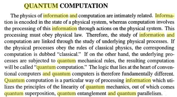
The first and second quantum revolutions:

Quantum 1.0

There are many devices available today which are fundamentally reliant on the effects of quantum mechanics. These include: laser systems, transistors and semi-conductor devices and other devices, such as MRI imagers. The phenomenon of magnetic resonance is rooted in the existence of spin angular momentum of a quantum system and its specific orientation with respect to an applied magnetic field. These devices are often referred to belonging to the ‘first quantum revolution’; the UK Defence Science and Technology Laboratory (Dstl) grouped these devices as ‘quantum 1.0, that is devices which rely on the effects of quantum mechanics. Put simply, no quantum, no internet. (And also no mobile phones, no videogames, no Facebook… you get the idea!). Thanks to Quantum 1.0, we were able to build devices whose functionalities extended beyond the capabilities of classical physics: lasers, digital cameras, modern medical instruments, and even nuclear power plants.

Quantum 2.0

Arguably, however, the most mind-boggling effects of quantum mechanics — such as entanglement — played little to no part in the first revolution. What sparked Quantum 2.0 was the marriage between quantum physics and information theory. Information theory, fathered by Claude Shannon after the second world war, is the mathematical theory that describes how information is processed, stored, and communicated. Quantum information theory explores the same concepts within the context of quantum systems. While the underlying goal of the theories is analogous, quantum information theory has a richer set of resources at its disposal. Quantum technologies are often described as the ‘second quantum revolution’ or ‘quantum 2.0. These are generally regarded as a class of device that actively create, manipulate and read out quantum states of matter, often using the quantum effects of superposition and entanglement. Quantum 2.0 is expected to be highly disruptive in three major domains: communication, measurement and sensing, and computation.

Quantum communication is best known as the science of sharing information in a completely secure way. In this sense, quantum technologies promise the creation of a quantum network where malicious users cannot access private information. In a recent pivotal experiment, Chinese and Austrian scientists used a satellite to exchange quantum-protected information between Beijing and Vienna, paving the way towards a large-scale quantum internet.

Quantum sensing and metrology exploit effects unique to quantum systems, such as entanglement, to realise measurements with greater precision than is possible with classical measuring devices. Applications include quantum magnetometers to detect tiny variations of magnetic fields (think of fancy compasses), atomic clocks (clocks that do not drift, and which tick many billions of times a second), and quantum-enhanced lidar (a widely used surveying and navigation method, with applications in fields as diverse as archaeology, agriculture, and autonomous vehicle guidance).

Last but not least — is quantum computing. Tech giants such as Google, IBM, Intel, and Microsoft, as well as startups such as Rigetti and Xanadu, are building the world’s first commercial quantum computers. These machines, first theorised by Yuri Manin and Richard Feynman in the early 80s, promise to outperform the best classical supercomputers for many important tasks. While the near-term utility of prototypical quantum processors is unclear, in the long run, fully-fledged universal quantum computers will be used to solve currently intractable problems. These include simulation of quantum systems (e.g. for drug and material design), studying chemical reactions (e.g. better catalysts for fertilisers), and quantum machine learning and AI (e.g. improved pattern recognition).

_

Today’s computers—both in theory (Turing machines) and practice (PCs, HPCs, laptops, tablets, smartphones, …)—are based on classical physics. They are limited by locality (operations have only local effects) and by the classical fact that systems can be in only one state at the time. However, modern quantum physics tells us that the world behaves quite differently. A quantum system can be in a superposition of many different states at the same time, and can exhibit interference effects during the course of its evolution. Moreover, spatially separated quantum systems may be entangled with each other and operations may have “non-local” effects because of this. Quantum computation is the field that investigates the computational power and other properties of computers based on quantum-mechanical principles. An important objective is to find quantum algorithms that are significantly faster than any classical algorithm solving the same problem.

_

Classical computers, which include smartphones and laptops, encode information in binary “bits” that can either be 0s or 1s. In a quantum computer, the basic unit of memory is a quantum bit or qubit. Qubits are made using physical systems, such as the spin of an electron or the orientation of a photon. These systems can be in many different arrangements all at once, a property known as quantum superposition. Qubits can also be inextricably linked together using a phenomenon called quantum entanglement. The result is that a series of qubits can represent different things simultaneously. For instance, eight bits is enough for a classical computer to represent any number between 0 and 255. But eight qubits is enough for a quantum computer to represent every number between 0 and 255 at the same time. A few hundred entangled qubits would be enough to represent more numbers than there are atoms in the universe.

This is where quantum computers get their edge over classical ones. In situations where there are a large number of possible combinations, quantum computers can consider them simultaneously. Examples include trying to find the prime factors of a very large number or the best route between two places. However, there may also be plenty of situations where classical computers will still outperform quantum ones. So the computers of the future may be a combination of both these types.

For now, quantum computers are highly sensitive: heat, electromagnetic fields and collisions with air molecules can cause a qubit to lose its quantum properties. This process, known as quantum decoherence, causes the system to crash, and it happens more quickly the more particles that are involved. Quantum computers need to protect qubits from external interference, either by physically isolating them, keeping them cool or zapping them with carefully controlled pulses of energy. Additional qubits are needed to correct for errors that creep into the system.

_

Classical computing relies on binary information, represented by bits that are either 1s or 0s. Qubits are fundamental to quantum computing and are somewhat analogous to bits in a classical computer. Quantum bits (or “qubits”) are made of subatomic particles, namely individual photons or electrons. Because these subatomic particles conform more to the rules of quantum mechanics than classical mechanics, they exhibit the bizarre properties of quantum particles. Qubits can be in a 1 or 0 quantum state. But they can also be in a superposition of the 1 and 0 states. This can be done using the magnetic spin of electrons, for example, which can be ‘up’, ‘down’ or some combination of up and down. This combination quantum state, known as a ‘superposition’, is the first of several concepts that form the foundation of the second quantum revolution. Superposition is the ability of a quantum system to be in multiple states simultaneously. The go-to example of superposition is the flip of a coin, which consistently lands as heads or tails—a very binary concept. However, when that coin is in mid-air, it is both heads and tails and until it lands, heads and tails simultaneously. Before measurement, the electron exists in quantum superposition.  A qubit only ‘chooses’ one state or the other – at random, though the probability depends on how much up and down are in the superposition – when it is measured. Until then qubits inside a quantum computer can effectively perform multiple calculations simultaneously. However, when qubits are measured the result is always either a 0 or a 1; the probabilities of the two outcomes depends on the quantum state they were in.

The second important concept is entanglement, where the behaviour of distant particles can be inextricably connected – or ‘entangled’. When one entangled particle is measured – and hence ‘chooses’ a state – its partner is immediately bound by that choice, no matter how far away it is. Entanglement is the key to quantum communication. When the two particles are entangled, the change in state of one particle will alter the state of its partner in a predictable way, which comes in handy when it comes time to get a quantum computer to calculate the answer to the problem you feed it. Quantum entanglement play an important role in the observed computational speed-up of some quantum algorithms. It is proved that entanglement is involved in quantum algorithms, such as Grover’s and Shor’s algorithms.

The third concept is the ‘no-cloning theorem’, which says the information in a quantum particle can never be fully copied without changing the state of the particle. A hacker can make a copy of your email now without you ever knowing; a hack of a quantum system, however, is bound by the laws of physics to leave traces.

Together, these phenomena pave the way for quantum computers able to crunch through big data problems that involve finding optimum solutions from vast numbers of options. That includes efficiently reverse-engineering the encryption keys that protect your internet banking sessions. At the same time, they make possible hack-proof quantum communication, in which eavesdropping can always be detected.

_

Imagine the following example, I write an Z on a random page in a random book in a library with 1 million books and tell a quantum and classical computer to find the Z. For a classical computer, it would have to sort through every page of every book one by one to find the Z which would consume a lot of time. For a quantum computer, a qubit in superposition can be in a multiple places at once so it can analyze every page at the same time and find the Z instantly.

Think about a phone book, and then imagine you have a specific number to look up in that phone book. A classical computer will search each line of the phone book, until it finds and returns the match. In theory, a quantum computer could search the entire phone book instantaneously, assessing each line simultaneously and returning the result much faster than a classical computer. These problems, which require the best combination of variables and solutions, are often called optimization problems. They are some of the most complex problems in the world, with potentially game-changing benefits.

Imagine you are building the world’s tallest skyscraper, and you have a budget for the construction equipment, raw materials, and labor, as well as compliance requirements. The problem you need to solve is how to determine the optimum combination of equipment, materials, and labor, etc. to maximize your investment. Quantum computing could help factor in all these variables to help us most efficiently plan for massive projects.

Optimization problems are faced across industries including software design, logistics, finance, web search, genomics, and more. While the toughest optimization problems in these industries stump classical computers, they are well-suited for being solved on a quantum machine.

_

Superposition and entanglement in a quantum computer mean:

1. Qubits unlike classical computers can be in a superposition of both 0 and 1
2. A complex system of qubits can be in many superpositions at once, example 5 qubits can be in a superposition of 32 states (2⁵ = 32)
3. Two entangled qubits are correlated with one another, information on one qubit will reveal information about the other unknown qubit.

The state of superposition, which is necessary to perform calculations, is difficult to achieve and enormously hard to maintain. Physicists use laser and microwave beams to put qubits in this working state and then employ an array of techniques to preserve it from the slightest temperature fluctuations, noises and electromagnetic waves. Current quantum computers are extremely error-prone due to the fragility of the working condition, which dissipates in a process called decoherence before most operations can be executed.

Quantum computational power is determined by how many qubits a machine can simultaneously leverage. Starting with a humble two qubits achieved in the first experiments in the late 1990s, the most powerful quantum computer today, operated by Google, can use up to 72 qubits.

_

Instead of being 1 or 0, qubit can be a bit of both. For instance, in layman’s terms, it can be in the superposition state 25%|0> + 75%|1>. We use the notation |0> and |1> to remember these are quantum states now. More generally, the state of a qubit is ⍺|0> + β|1>, where ⍺ and β are complex numbers called the amplitudes. With 2 qubits you can have the four combinations |00>, |01>, |10> and |11> at the same time. 8 combinations with 3 qubits, and so on, always existing in parallel. That’s quantum physics! A qubit can be an atom, a photon, an electron, an ion, or any quantum system that can have two states.

So the input of a quantum algorithm is made of qubits. If you have n qubits, you have simultaneously 2ⁿ configurations. With 300 qubits you have 2³⁰⁰ states, this is number of atoms in the universe!

Another important fact: if you measure a set of qubits, you won’t see the whole superposition (you’re not quantum), but just one of the configurations, at random, with a probability related to the amplitude of this configuration.

_

How exponential speed-up over classical computers might come from?

Classically, the time it takes to do certain computations can be decreased by using parallel processors. To achieve an exponential decrease in time requires an exponential increase in the number of processors, and hence an exponential increase in the amount of physical space needed. However, in quantum systems the amount of parallelism increases exponentially with the size of the system. Thus, an exponential increase in parallelism requires only a linear increase in the amount of physical space needed.

The input to a quantum computation can be put in a superposition state that encodes all possible input values. Performing the computation on this initial state will result in superposition of all of the corresponding output values. Thus, in the same time it takes to compute the output for a single input state on a classical computer, a quantum computer can compute the values for all input states. This process is known as quantum parallelism. However, measuring the output states will randomly yield only one of the values in the superposition, and at the same time destroy all of the other results of the computation.

While a quantum system can perform massive parallel computation, access to the results of the computation is restricted. Accessing the results is equivalent to making a measurement, which disturbs the quantum state. This problem makes the situation, on the face of it, seem even worse than the classical situation; we can only read the result of one parallel thread, and because measurement is probabilistic, we cannot even choose which one we get.

A conventional computer processes information by encoding it into 0s and 1s. If we have a sequence of thirty 0s and 1s, it has about one billion of possible values. However, a classical computer can only be in one of these one billion states at the same time. A quantum computer can be in a quantum combination of all of those states, called superposition. This allows it to perform one billion or more copies of a computation at the same time. In a way, this is similar to a parallel computer with one billion processors performing different computations at the same time—with one crucial difference. For a parallel computer, we need to have one billion different processors. In a quantum computer, all one billion computations will be running on the same hardware. This is known as quantum parallelism.

The result of this process is a quantum state that encodes the results of one billion computations. The challenge for a person who designs algorithms for a quantum computer is: how do we access these billion results? If we measured this quantum state, we would get just one of the results. All of the other 999,999,999 results would disappear.

To solve this problem, one uses the second effect, quantum interference. Consider a process that can arrive at the same outcome in several different ways. In the non-quantum world, if there are two possible paths toward one result and each path is taken with a probability ¼, the overall probability of obtaining this result is ¼+¼= ½. Quantumly, the two paths can interfere, increasing the probability of success to 1.

Quantum algorithms combine these two effects. Quantum parallelism is used to perform a large number of computations at the same time, and quantum interference is used to combine their results into something that is both meaningful and can be measured according to the laws of quantum mechanics.

In the past few years, various people have found clever ways of finessing the measurement problem to exploit the power of quantum parallelism. This sort of manipulation has no classical analog, and requires non-traditional programming techniques. One technique manipulates the quantum state so that a common property of all of the output values such as the symmetry or period of a function can be read off. This technique is used in Shor’s factorization algorithm. Another technique transforms the quantum state to increase the likelihood that output of interest will be read. Grover’s search algorithm makes use of such an amplification technique.

Unlike classical bits, a quantum bit can be put in a superposition state that encodes both 0 and 1. There is no good classical explanation of superpositions: a quantum bit representing 0 and 1 can neither be viewed as “between” 0 and 1 nor can it be viewed as a hidden unknown state that represents either 0 or 1 with a certain probability. Even single quantum bit enables interesting application like secure key distribution. But the real power of quantum computation derives from the exponential state spaces of multiple quantum bits: just as a single qubit can be in a superposition of 0 and 1, a register of n qubits can be in a superposition of all 2^n possible values.

_

Microsoft researcher David Reilly:

“A quantum machine is a kind of analog calculator that computes by encoding information in the ephemeral waves that comprise light and matter at the nanoscale.”

Rebecca Krauthamer, CEO of quantum computing consultancy Quantum Thought, compares quantum computing to a crossroads that allows a traveller to take both paths. “If you’re trying to solve a maze, you’d come to your first gate, and you can go either right or left,” she said. “We have to choose one, but a quantum computer doesn’t have to choose one. It can go right and left at the same time.” “It can, in a sense, look at these different options simultaneously and then instantly find the most optimal path,” she said. “That’s really powerful.”

_

The Turing machine, developed by Alan Turing in the 1930s, is a theoretical device that consists of tape of unlimited length that is divided into little squares. Each square can either hold a symbol (1 or 0) or be left blank. A read-write device reads these symbols and blanks, which gives the machine its instructions to perform a certain program. In a quantum Turing machine, the difference is that the tape exists in a quantum state, as does the read-write head. This means that the symbols on the tape can be either 0 or 1 or a superposition of 0 and 1; in other words the symbols are both 0 and 1 (and all points in between) at the same time. While a normal Turing machine can only perform one calculation at a time, a quantum Turing machine can perform many calculations at once.

Today’s computers, like a Turing machine, work by manipulating bits that exist in one of two states: a 0 or a 1. Quantum computers aren’t limited to two states; they encode information as quantum bits, or qubits, which can exist in superposition. Qubits represent atoms, ions, photons or electrons and their respective control devices that are working together to act as computer memory and a processor. Because a quantum computer can contain these multiple states simultaneously, it has the potential to be millions of times more powerful than today’s most powerful supercomputers.

This superposition of qubits is what gives quantum computers their inherent parallelism. According to physicist David Deutsch, this parallelism allows a quantum computer to work on a million computations at once, while your desktop PC works on one. A 30-qubit quantum computer would equal the processing power of a conventional computer that could run at 10 teraflops (trillions of floating-point operations per second). Today’s typical desktop computers run at speeds measured in gigaflops (billions of floating-point operations per second).

Quantum computers also utilize another aspect of quantum mechanics known as entanglement. One problem with the idea of quantum computers is that if you try to look at the subatomic particles, you could bump them, and thereby change their value. If you look at a qubit in superposition to determine its value, the qubit will assume the value of either 0 or 1, but not both (effectively turning your quantum computer into a digital computer). To make a practical quantum computer, scientists have to devise ways of making measurements indirectly to preserve the system’s integrity. Entanglement provides a potential answer. In quantum physics, if you apply an outside force to two atoms, it can cause them to become entangled, and the second atom can take on the properties of the first atom. So if left alone, an atom will spin in all directions. The instant it is disturbed it chooses one spin, or one value; and at the same time, the second entangled atom will choose an opposite spin, or value. This allows scientists to know the value of the qubits without actually looking at them.

_

Computer scientists control the microscopic particles that act as qubits in quantum computers by using control devices.

-Ion traps use optical or magnetic fields (or a combination of both) to trap ions.

-Optical traps use light waves to trap and control particles.

-Quantum dots are made of semiconductor material and are used to contain and manipulate electrons.

-Superconducting circuits allow electrons to flow with almost no resistance at very low temperatures.

_

Quantum computing is the use of quantum-mechanical phenomena such as superposition and entanglement to perform computation. A quantum computer is used to perform such computation, which can be implemented theoretically or physically. There are two main approaches to physically implementing a quantum computer currently, analog and digital. Analog approaches are further divided into quantum simulation and adiabatic quantum computation. Digital quantum computers use quantum logic gates to do computation. Both approaches use quantum bits or qubits. Digital quantum computing paradigm offers highly desirable features such as universality, scalability, and quantum error correction. However, physical resource requirements to implement useful error-corrected quantum algorithms are prohibitive.

Universal quantum computers are based on logical gates and work similar to the underlying logic foundations of classical computers. Hence, universal quantum computers are extremely useful for computing problems improving on our current knowledge base of solutions. Universal quantum computers are the most powerful and most generally applicable, but also the hardest to build. A truly universal quantum computer would likely make use of over 100,000 qubits — some estimates put it at 1 million qubits. Remember that today, the most qubits we can access is not even 128. The basic idea behind the universal quantum computer is that you could direct the machine at any massively complex computation and get a quick solution.

Adiabatic computers are analog, but are easier to produce. These are more relaxed with respect to qubit state stability. Hence, it is easier to produce 1000s of qubits on adiabatic computers. However, adiabatic computers can be used for limited use cases such as optimisation problems.

_

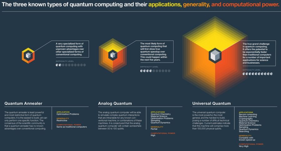
The first small 2-qubit quantum computer was built in 1997 and in 2001 a 5-qubit quantum computer was used to successfully factor the number 15. Since then, experimental progress on a number of different technologies has been steady but slow. Currently, the largest quantum computers (based on superconducting qubits or ion-trap qubits) have a few dozen qubits.

The practical problems facing physical realizations of quantum computers seem formidable. The problems of noise and decoherence have to some extent been solved in theory by the discovery of quantum error-correcting codes and fault-tolerant computing, but these problems are by no means solved in practice. On the other hand, we should realize that the field of physical realization of quantum computing is still in its infancy and that classical computing had to face and solve many formidable technical problems as well—interestingly, often these problems were even of the same nature as those now faced by quantum computing (e.g., noise-reduction and error-correction). Moreover, while the difficulties facing the implementation of a full quantum computer may seem daunting, more limited applications involving quantum communication have already been implemented with some success, for example teleportation (which is the process of sending qubits using entanglement and classical communication), and quantum cryptography is nowadays even commercially available.

Even if the theory of quantum computing never materializes to a real large-scale physical computer, quantum-mechanical computers are still an extremely interesting idea which will bear fruit in other areas than practical fast computing. On the physics side, it may improve our understanding of quantum mechanics. The emerging theory of entanglement has already done this to some extent. On the computer science side, the theory of quantum computation generalizes and enriches classical complexity theory and may help resolve some of its problems.

_

Classical computing has been the backbone of modern society. It gave us satellite TV, the internet and digital commerce. It put robots on Mars and smartphones in our pockets. But many of the world’s biggest mysteries and potentially greatest opportunities remain beyond the grasp of classical computers. To continue the pace of progress, we need to augment the classical approach with a new platform, one that follows its own set of rules. That is quantum computing.

Classical computers are better at some tasks than quantum computers (email, spreadsheets and desktop publishing to name a few). Quantum computers will never “replace” classic computers, simply because there are some problems that classic computers are better and/or more efficient at solving. A likely future scenario is that quantum computing will augment subroutines of classical algorithms that can be efficiently run on quantum computers, such as sampling, to tackle specific business problems. For instance, a company seeking to find the ideal route for retail deliveries could split the problem into two parts and leverage each computer for its strengths.

The intent of quantum computers is to be a different tool to solve different problems, not to replace classical computers. Quantum computers are great for solving optimization problems from figuring out the best way to schedule flights at an airport to determining the best delivery routes for the FedEx truck. There are some problems so difficult, so incredibly vast, that even if every supercomputer in the world worked on the problem, it would still take longer than the lifetime of the universe to solve. Quantum computers hold the promise to solve some of our planet’s biggest challenges – in environment, agriculture, health, energy, climate, materials science, and problems we’ve not yet even imagined. The impact of quantum computers will be far-reaching and have as great an impact as the creation of the transistor in 1947, which paved the way for today’s digital economy.

Every day, we produce 2.5 exabytes of data. That number is equivalent to the content on 5 million laptops. Quantum computers will make it possible to process the amount of data we’re generating in the age of big data. According to Professor Catherine McGeoch at Amherst University, a quantum computer is “thousands of times” faster than a conventional computer. Rather than use more electricity, quantum computers will reduce power consumption anywhere from 100 up to 1000 times because quantum computers use quantum tunneling. In order to keep quantum computers stable, they need to be cold. That’s why the inside of D-Wave Systems’ quantum computer is -460 degrees Fahrenheit. Quantum computers are very fragile. Any kind of vibration impacts the atoms and causes decoherence.

There are several algorithms already developed for quantum computers including Grover’s for searching an unstructured database and Shor’s for factoring large numbers. Once a stable quantum computer gets developed, expect that machine learning will exponentially accelerate even reducing the time to solve a problem from hundreds of thousands of years to seconds. Remember when IBM’s computer Deep Blue defeated chess champion, Garry Kasparov in 1997.  It was able to gain a competitive advantage because it examined 200 million possible moves each second. A quantum machine would be able to calculate 1 trillion moves per second!

_

The most important benefit of quantum computers is the speed at which it can solve complex problems. While they’re lightning quick at what they do, they don’t provide capabilities to solve problems from undecidable or NP Hard problem classes. There is a problem set that quantum computing will be able to solve, however it’s not applicable for all computing problems. Typically, the problem set that quantum computers are good at solving involves number or data crunching with a huge amount of inputs, such as “complex optimization problems and communication systems analysis problems” — calculations that would typically take supercomputers days, years, even billions of years to brute force.

The application that’s regularly trotted out as an example that quantum computers will be able to instantly solve is strong RSA encryption. A recent study by the Microsoft Quantum Team suggests this could well be the case, calculating that it’d be doable with around a 2330 qubit quantum computer.

The most cutting edge quantum computers built by heavyweights like Intel, Microsoft, IBM all are currently hovering at around the 50 qubit mark, however Google have recently announced Bristlecone, their 72-qubit project. Given Moore’s law and the current speed of development of these systems, strong RSA may indeed be cracked within 10 years.

_

Quantum computers working with classical systems have the potential to solve complex real-world problems such as simulating chemistry, modelling financial risk and optimizing supply chains.  For example, Exxon Mobil plans to use quantum computing to better understand catalytic and molecular interactions that are too difficult to calculate with classical computers. Potential applications include more predictive environmental models and highly accurate quantum chemistry calculations to enable the discovery of new materials for more efficient carbon capture.  JP Morgan Chase is focusing on use cases for quantum computing in the financial industry, including trading strategies, portfolio optimisation, asset pricing and risk analysis.

_

Pharmaceutical companies have an abiding interest in enzymes. These proteins catalyze all kinds of biochemical interactions, often by targeting a single type of molecule with great precision. Harnessing the power of enzymes may help alleviate the major diseases of our time. Unfortunately, we don’t know the exact molecular structure of most enzymes. In principle, chemists could use computers to model these molecules in order to identify how the molecules work, but enzymes are such complex structures that most are impossible for classical computers to model. A sufficiently powerful quantum computer, however, could accurately predict in a matter of hours the properties, structure, and reactivity of such substances—an advance that could revolutionize drug development and usher in a new era in healthcare. Quantum computers have the potential to resolve problems of this complexity and magnitude across many different industries and applications, including finance, transportation, chemicals, and cybersecurity.

Solving the impossible in a few hours of computing time, finding answers to problems that have bedeviled science and society for years, unlocking unprecedented capabilities for businesses of all kinds—those are the promises of quantum computing, a fundamentally different approach to computation.

_

To be clear, quantum computing is expected to be designed to work alongside classical computers, not replace them.  Quantum computers are large machines that require their qubits to be kept near absolute zero (minus 273 degrees Celsius) in temperature, so don’t expect them in your smartphones or laptops. And rather than the large number of relatively simple calculations done by classical computers, quantum computers are only suited to a limited number of highly complex problems with many interacting variables.

______

______

Basics of quantum computing:

_

These concepts will give you a good introduction to the fundamental knowledge you need to start coding quantum programs.

1. Basic quantum mechanics: Some basic concepts of quantum mechanics and its mathematical notation will be helpful to understand quantum programming.
2. Linear algebra (vectors and matrices): In quantum computing, quantum states are represented by vectors, with quantum operations being linear transformations applied to these vectors.
3. Complex arithmetic: The coefficients of quantum state vectors are complex numbers. You can understand some basic quantum computing concepts without them, but you won’t get far before you need to incorporate them into your quantum toolkit. You need to learn complex arithmetic that explains some of the mathematical background required to work with quantum computing.

_

Quantum mechanics, which is the underlying foundation for quantum computing, is heavily based on the use of linear algebra for describing quantum states in terms of wave functions as linear combinations of basis states with probability amplitudes, such that the sum of the probabilities for all states is exactly 1.0 by definition.

The question is whether or to what degree the designers of quantum algorithms need to know any or much of quantum mechanics and linear algebra to design great quantum algorithms. The jury is still out as to how much knowledge of quantum mechanics and linear algebra is needed by quantum computing practitioners. The answer is likely to be some, so the question will be how to make a small subset of quantum mechanics and linear algebra approachable, comprehendible, and palatable to the broad audience of designers of quantum algorithms and quantum programs without requiring them to rise to the knowledge level of a theoretical physicist.

_

Wave function:

As noted earlier, the basis of quantum computing is the quantum wave function. It represents the complete state of the quantum computer, in terms of probabilities for each of the quantum states. The wave function is what enables superposition and even entanglement. In quantum mechanics and quantum computing we speak of a wave function which represents the complete state of a quantum system, either a single qubit or two qubits which are entangled. Actually, there is a separate wave function for each qubit or pair of entangled qubits. A quantum wave function is a mathematical formulation of the states of a quantum system. The individual states of a quantum system are known as basis states or basis vectors. For qubits there are two basis states — |0> and |1>, which are indeed each comparable to the classical binary values of 0 and 1. But basis states are not quite the same as binary values. They are the actual states of the underlying quantum system, the physical qubit. There are a variety of techniques for realizing qubits, quantum spin being one of the most popular these days. Spin has physical values of up and down, which correspond to the voltage levels of transistors, classical logic gates, and classical flops, but the point is that those voltage levels or magnetic intensities of storage media correspond to bits rather than being the bits themselves. And spin differs since it can be superimposed and entangled.

The only real downside is that you cannot examine the wave function of a quantum system (each qubit or pair of entangled qubits) without causing it to collapse. Collapse of the wave function is not a complete loss, since it collapses into a specific value or 0 or 1 for each qubit which you attempt to observe or measure, but you do lose the probability values (called probability amplitudes) for each of the superimposed or entangled quantum states of the qubit.

_

Quantum states:

Much is made of the concept that a quantum computer with n qubits can represent and operate on 2^n distinct and superimposed quantum states, all at the same time. A 4-qubit machine has 16 states, an 8-qubit machine has 256 states, a 20-qubit machine has over one million states, and a machine with more than 32 qubits has more states than you can even count in a 32-bit integer on a classical computer. The power of these qubits is their inherent ability to scale exponentially so that a two-qubit machine allows for four calculations simultaneously, a three-qubit machine allows for eight calculations, and a four-qubit machine performs 16 simultaneous calculations.

_

Quantum computers are probabilistic rather than strictly deterministic:

One of the great qualities of a classical computer, based on the concept of a Turing machine, is that it is strictly deterministic. You can mimic nondeterminism, such as generating random numbers, but that’s the exception rather than the norm. Quantum computers on the other hand are inherently probabilistic rather than deterministic, just as with the quantum mechanics upon which quantum computing is based. This distinction requires a significant, radical change in mindset for the design of algorithms and code for a quantum computer. Rather than calculating the answer to a problem as a classical computation would do, a quantum computation generates the probabilities for any number of possible solutions. Analogously to a classical Turing machine, a quantum program can mimic determinism, but that is failing to exploit the power of the quantum computer.

_

Qubits and Superposition:

The ordinary bits we use in typical digital computers are either 0 or 1. You can read them whenever you want, and unless there is a flaw in the hardware, they won’t change. Qubits aren’t like that. They have a probability of being 0 and a probability of being 1, but until you measure them, they may be in an indefinite state. That state, along with some other state information that allows for additional computational complexity, can be described as being at an arbitrary point on a sphere (of radius 1), that reflects both the probability of being measured as a 0 or 1 (which are the north and south poles).

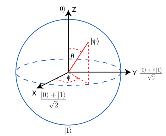
The Bloch sphere is used to represent the possible states of a single qubit.

The qubit’s state is a combination of the values along all three axes. This is called superposition. Some texts describe this property as “being in all possible states at the same time,” while others think that’s somewhat misleading (between 0 and 1) and that we’re better off sticking with the probability explanation. Either way, a quantum computer can actually do math on the qubit while it is in superposition — changing the probabilities in various ways through logic gates — before eventually reading out a result by measuring it. In all cases, though, once a qubit is read, it is either 1 or 0 and loses its other state information.

Qubits typically start life at 0, although they are often then moved into an indeterminate state using a Hadamard Gate, which results in a qubit that will read out as 0 half the time and 1 the other half. Other gates are available to flip the state of a qubit by varying amounts and directions — both relative to the 0 and 1 axes, and also a third axis that represents phase, and provides additional possibilities for representing information. The specific operations and gates available depend on the quantum computer and toolkit you’re using.

Entanglement is where the action is:

Groups of independent qubits, by themselves, aren’t enough to create the massive breakthroughs that are promised by quantum computing. The magic really starts to happen when the quantum physics concept of entanglement is implemented. One industry expert likened qubits without entanglement as being a “very expensive classical computer.” Entangled qubits affect each other instantly when measured, no matter far apart they are, based on what Einstein euphemistically called “spooky action at a distance.” In terms of classic computing, this is a bit like having a logic gate connecting every bit in memory to every other bit.

You can start to see how powerful that might be compared with a traditional computer needing to read and write from each element of memory separately before operating on it. As a result, there are multiple large potential gains from entanglement. The first is a huge increase in the complexity of programming that can be executed, at least for certain types of problems. One that’s creating a lot of excitement is the modeling of complex molecules and materials that are very difficult to simulate with classical computers. Another might be innovations in long-distance secure communications — if and when it becomes possible to preserve quantum state over large distances. Programming using entanglement typically starts with the C-NOT gate, which flips the state of an entangled particle if its partner is read out as a 1. This is sort of like a traditional XOR gate, except that it only operates when a measurement is made.

_

Parallel positions:

Qubits don’t represent data in the same way as bits. Because qubits in superposition are both 0 and 1 at the same time, they can similarly represent all possible answers to a given problem simultaneously. This is called quantum parallelism, and it’s one of the properties that makes quantum computers so much faster than classical systems.

The difference between classical computers and their quantum counterparts could be compared to a situation in which there is a book with some pages randomly printed in blue ink instead of black. The two computers are given the task of determining how many pages were printed in each color. A classical computer would go through every page. Each page would be marked, one at a time, as either being printed in black or in blue. A quantum computer, instead of going through the pages sequentially, would go through them all at once. Once the computation was complete, a classical computer would give you a definite, discrete answer. If the book had three pages printed in blue, that’s the answer you’d get.

But a quantum computer is inherently probabilistic. This means the data you get back isn’t definite. In a book with 100 pages, the data from a quantum computer wouldn’t be just three. It also could give you, for example, a 1 percent chance of having three blue pages or a 1 percent chance of 50 blue pages. An obvious problem arises when trying to interpret this data. A quantum computer can perform incredibly fast calculations using parallel qubits, but it spits out only probabilities, which, of course, isn’t very helpful – unless, that is, the right answer could somehow be given a higher probability.

Interference:

Consider two water waves that approach each other. As they meet, they may constructively interfere, producing one wave with a higher crest. Or they may destructively interfere, cancelling each other so that there’s no longer any wave to speak of. Qubit states can also act as waves, exhibiting the same patterns of interference, a property, researcher can exploit to identify the most likely answer to the problem they’re given. If you can set up interference between the right answers and the wrong answers, you can increase the likelihood that the right answers pop up more than the wrong answers. You’re trying to find a quantum way to make the correct answers constructively interfere and the wrong answers destructively interfere.

When a calculation is run on a quantum computer, the same calculation is run multiple times, and the qubits are allowed to interfere with one another. The result is a distribution curve in which the correct answer is the most frequent response.

_

How superposition enables Quantum Computers:

Let’s say you’ve organized a dinner, and need to decide where to seat your guests. For simplicity’s sake, let’s say you only have 3 guests, and 2 tables to place them on.

The thing is, some of these guests don’t like each other, but others do.

Let’s say:

Person A and C are friends 😊

Person A and B are enemies ☹

Person B and C are enemies ☹

In this situation, you want to have the highest number of friends together, while having the lowest number of enemies together.

How this would work on a regular computer:

Well, we only have 2 tables, so we can assign tables to each guest in binary, with a 1 or 0. So we have Table 1, and Table 0. For example, one combination of placements could be:

001 (Person A and B are placed on Table 0, and Person C is placed on Table 1)

Here are all the possible combinations:

Person A	Person B	Person C
0	0	0
0	0	1
0	1	0
0	1	1
1	0	0
1	0	1
1	1	0
1	1	1

Now, we want to optimize for friends, and against enemies placed on the same table. With this knowledge, we can create a score algorithm. It could be something like this:

Score = (# Friends) – (# Enemies)

With this metric, the scores would be:

Person A	Person B	Person C	Score	Result
0	0	0	-1	☹
0	0	1	-1	☹
0	1	0	1	😊
0	1	1	-1	☹
1	0	0	-1	☹
1	0	1	1	😊
1	1	0	-1	☹
1	1	1	-1	☹

As you can tell, there are 2 arrangements which would lead to the highest score: 010 & 101.

In this situation, a conventional computer would have to try out all of these configurations separately using 3 bits (one at a time) and compute each score. Then select the highest.

Now of course, this is a really simple problem which would take almost no time on a conventional computer. However, what if we increased the number of people?

With 3 people, there are 8 (2x2x2 = 2³) configurations.

With 20 people, there are 1048576 (2²⁰) configurations.

With 200 people, there are 2²⁰⁰ combinations!

That’s about 10⁶⁰ or 10 with 60 zeros behind it.

The world’s fastest computers can only compute 200,000 trillion calculations per second. Meaning it would take ~10⁴⁶ seconds, which is way too long. Actually longer than the age of the universe.

How this would work on a Quantum Computer:

Remember there are 8 possible combinations:

Person A	Person B	Person C
0	0	0
0	0	1
0	1	0
0	1	1
1	0	0
1	0	1
1	1	0
1	1	1

With a conventional computer, we had to compute each combination separately, one at a time. And that’s where quantum computers pull ahead. With a quantum computer, we can compute all of these scores at one time, using 3 qubits by utilizing 3 qubits in superposition, so we are effectively creating 8 parallel realities.

When you set a qubit to a superposition of both 1 and 0, you are basically unravelling 2 parallel realities, do this for all 3 qubits, and you have 8. In each reality, the combinations of qubits are different, meaning each combination exists in one of the parallel realities. When you apply your computations to the qubits, the computation actually unravels over all 8 realities in parallel, meaning at the same time. This is how we get an exponential speed up!

After computing the final scores, we select the reality with the optimized score, and continue along that timeline. In other words, the realities collapses into the optimized state. Just like probability distributions are in multiple states, but collapse into one state after you measure the outcome.

Now what if we increased the number of people?

Well, all we need is the same number of qubits, as there are people. 3 people requires 3 qubits, 200 people requires 200 qubits.

But as long as we have the same number of qubits, as there are people, we can solve these problems in 1 operation for any number of people. You can create 2²⁰⁰ parallel realities, apply the operation to each at the same time, and collapse them into the reality with the highest score.

But, there are errors when we do quantum computations.  In theory, we’d collapse to the optimal state (In this case 010 or 101) every time, but there are errors in quantum computers today, due to the fragility of qubits. To resolve this, we run the same operation numerous times on quantum computers, then select the best result. Errors become more prominent as the problems become more complex, so we repeat a variable amount of time.

Given these two things, your quantum computer will spit out one of the best solutions in a few milliseconds. In this case, that’s 001 or 110 with a score of 1.

Now, in theory, a quantum computer is able to find one of the best solutions every time it runs. However, in reality, there are errors when running a quantum computer. So, instead of finding the best solution, it might find the second-best solution, the third best solution, and so on. These errors become more prominent as the problem becomes more and more complex. So, in practice, you will probably want to run the same operation on a quantum computer dozens of times or hundreds of times. Then pick the best result out of the many results you get.

How a quantum computer scales:

Even with the errors mentioned, the quantum computer does not have the same scaling issue a regular computer suffers from.

When there are 3 people we need to divide into two tables, the number of operations we need to perform on a quantum computer is 1. This is because a quantum computer computes the score of all configurations at the same time.

When there are 4 people, the number of operations is still 1.

When there are 100 people, the number of operations is still 1.

With a single operation, a quantum computer computes the scores of all 2¹⁰⁰ ~= 10³⁰ = one million million million million million configurations at the same time.

As mentioned earlier, in practice, it’s probably best to run your quantum computer dozens of times or hundreds of times and pick the best result out of the many results you get.

However, it’s still much better than running the same problem on a regular computer and having to repeat the same type of computation one million million million million million times.

_

In a nutshell what is the fundamental difference between classical and quantum computing?

A bit (short for binary digit) is the smallest unit of data in a computer. A bit has a single binary value, either 0 or 1.  All calculations are done using these two values (0 and1) and all calculations are done sequentially one after another. In quantum computing there is qubit having value of 1 or 0 or both or all values between 0 and 1. Even single quantum bit enables interesting application like secure key distribution, and more complex calculations require more qubits, and all calculations are done simultaneously in one operation only no matter number of input variables. As number of qubits increases, the computing power increases exponentially. In classical computing as the number of transistors increases, the computing power increases linearly and not exponentially. Bits are on or off voltage/current in transistor but qubit is mathematical wave function of electron spin or photon polarization.

__

The ‘EPR’ paradox and quantum entanglement:

As is well known, Einstein was suspicious of the probabilities inherent in quantum mechanics. In the famous ‘Bohr-Einstein debate’ he tried unsuccessfully to pinpoint an intrinsic contradiction in quantum theory. The climax of this debate was his formulation, with Podolsky and Rosen, of a situation in which one of the essential peculiarities of quantum mechanics was exposed.

Modern variant (due to Bohm) of the argument of Einstein, Podolsky and Rosen goes as follows. Imagine we have an elementary particle with zero charge and spin – such as a neutral pion – at rest, which then disintegrates into a spin 1/2 electron and a spin 1/2 positron (figure below). Since angular momentum is conserved in this decay, the two spin half particles must together combine to form a spin zero state. Thus if we measure the electron spin to be up, for example, we know that the positron spin must be down – and vice versa.

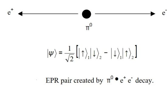
So what is the problem? Well, the electron and positron are separating rapidly in opposite directions (conservation of linear momentum). If we make the first spin measurement on the electron, we could in principle measure the positron spin before even a light signal had time to communicate to the positron whether its spin has to be up or down! In fact, no matter what we do, we always find perfect anti-correlation between the spins, even though there could have been no physical communication between the two particles. Einstein thought that this demonstrated that the spins of the two particles are therefore not indeterminate before measurement but are actually ‘elements of physical reality’. According to Bohr’s ‘Copenhagen’ interpretation of quantum mechanics, it is meaningless to talk of the spin direction of the particles until you make a measurement. This is the truly startling point about quantum mechanics: orthodoxy has it that there is no objective reality (a reality independent of an ‘observer’) for the electrons and their spins! Einstein would have none of this and thought that things must really be predetermined in advance of the measurement. In other words, although our present formulation of quantum mechanics has the spins as only having a probabilistic value, and since ‘spooky, faster than light’ signaling is out of the question, there must be some ‘hidden variables’ that make the directions of the spins predetermined from the outset. After several months of frantic activity devising a response to Einstein’s challenge, Bohr declared the EPR paradox not to be a paradox at all and argued essentially that quantum mechanics demands that you are only allowed to treat the electron-positron system as a single quantum system. And there the matter rested, as a rather abstract and philosophical debate about hidden variables and objective reality – since neither side denied that quantum mechanics worked as a predictive framework. Until John Bell entered the debate.

John Bell’s great contribution was to devise a way of putting these two views – hidden variables/objective reality and quantum mechanics/no objective reality – to an experimental test. In our discussion above, we only discussed measuring spins in the ‘up’ and ‘down’ direction. What happens if we measure ‘up/down’ for the electron but ‘left/right’ for the positron. This is easy to calculate according to quantum mechanics. If the electron is found to be ‘up’, the positron state must be ‘down’ for our zero spin initial state, and by standard quantum mechanics a down state may be written as an equal superposition of ‘left’ and ‘right’ eigenstates. Thus a measurement of the ‘right/left’ kind on the positron would yield right or left with equal probabilities. John Bell’s contribution was to consider the correlations predicted for spin measurements not at right angles but at an angle of 37 degrees, say. In this case, the probabilities for ‘up’ and ‘down’ along this new direction are now not equal and are not purely random. What Bell was able to prove was that the correlations predicted by quantum mechanics are greater than could be obtained from any local hidden variable theory – where local means there is no faster than light signaling or any other peculiar, acausal behaviour. Unfortunately for Einstein, Alain Aspect and co-workers, in a famous series of experiments, demonstrated that Nature appears to obey quantum mechanics.

Why have I made this apparent diversion to discuss the EPR paradox? The reason is that the EPR state of the electron and positron is an example of an ‘entangled state’.

In the EPR case these two particles are rapidly flying apart. The key point about an entangled state is that it is not possible to write such a state as a simple product state of particle 1 and particle 2. Particle 1 is not in a definite spin state – the spin information is shared between the two particles. This is an example of what is sometimes called an ‘entangled qubit’ or just an ‘e-bit’. The important thing to remember is that it is with such states that quantum mechanics shows its bizarre non-local power.

It is the sharing of two halves of an entangled pair that makes possible such things as ‘quantum teleportation’. In this case, interacting with one half of an EPR pair affects the other half in a non-local way. This remarkable non-local nature of quantum mechanics is also an essential ingredient of quantum algorithms on quantum computers.

_

In a nutshell:

Quantum mechanics is weird. Quantum systems can generate weird patterns that are very hard to generate classically. But quantum systems can also learn and recognize weird patterns that can’t be recognized classically. And the reason that they can do this is that quantum computing and quantum mechanics is all about linear algebra. But with a very small number of quantum bits, we can have states that represent vectors in a very high-dimensional vector space. And then quantum computers can be used to do linear algebra operations such as fast Fourier Transforms, finding Eigenvectors and Eigenvalues, and inverting Matrices exponentially faster than we can do classically.

______

______

Optimization:

In mathematics and computer science, an optimization problem is the problem of finding the best solution from all feasible solutions. An optimization problem is essentially finding the best solution to a problem from endless number of possibilities. Classical computers would have to configure and sort through every possible solution one at a time, on a large-scale problem this could take millions of years. Quantum computers can find all possible variants at the same time using superposition and entanglement and sift through large amounts of input variables in a significantly small amount of time.

_

While classical computers can perfectly optimize small systems, they only find incremental improvements for large systems such as transportation routes and product pricing. This is due to their rapidly rising running time as a function of problem size.

Placement of logic gates on an integrated circuit is an example. Chip design tools have optimizers that place logic gates on a chip’s surface with just enough space between to hold the wiring that defines the chip’s function. Better placement reduces chip area—and hence cost— while simultaneously increasing the chip’s speed because the shorter wires convey information in less time. However, a chip might be profitable even if it’s a few percent larger than necessary, so perfect optimization isn’t essential.

Classical placement algorithms such as simulated annealing follow the same principle as raindrops trying to find the lowest elevation by flowing downhill. Figure below shows an energy landscape for water by position across the US. Water dropped almost anywhere will flow to an ocean. Oceans are low, but not as low as Death Valley. However, Death Valley has a small rainfall basin surrounded by high mountains, so a random raindrop would be unlikely to fall into its basin.

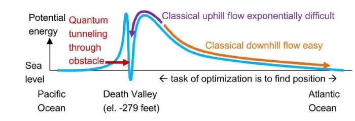
Figure above shows that optimization involves finding the lowest point on a potential energy curve (blue), which is Death Valley even though most water flows to the oceans. Classical optimization (orange) works like raindrops flowing downhill, but simulated annealing allows limited uphill movement (purple). However, quantum computer optimization can use a quantum physics principle called ‘tunneling’ to go through a high energy barrier (red).

Mathematicians, computer scientists, and programmers have improved simulated annealing so that potential solutions can jump over an obstacle, but the probability of this occurring decreases exponentially with the height of the jump. Human effort has also created heuristics, such as chip design tools that handle memories, busses, and clock lines in special ways.

One form of quantum machine learning uses “quantum tunneling” to go through the peak in figure above, with the probability of this occurring declining exponentially with the width of the peak. The tunneling approach may or may not be better than simulated annealing, but applying both techniques might give a better answer than either alone. Other quantum algorithms work quite differently, such as not using potential energy at all.

_

Let us say you have N applicants for acting, and you want to select 1 actor.

Option 1: Audition the N applicants, score them, and select the applicant with the highest score. If you take 1 hour for auditioning each applicant, this process will take N hours plus post-audition time.

Option 2: The public is aware about acting capabilities of the N applicants. Ask the public to cast their votes, and select the applicant with the highest vote. This process is likely to take about √N hours plus post-voting time.

Option 2 uses a community interaction and eliminates the need for one-to-one interactions, and thereby, reduces the required time from an order of N to an order of √N. This time reduction is significant for large N.

The bits of a classical computer behave in a deterministic and individualistic way. There is no “public of bits” knowing about other bits. As a result, sorting and other operations in a classical computer have to rely on something similar to option 1.

The qubits of a quantum computer behave in a probabilistic and interacting way. Due to wave nature of qubits, all qubits know about all other qubits, and thus, there is a “public of qubits” knowing about other qubits. As a result, sorting and other operations in a quantum computer can rely on something similar to option 2.

Thus, the “community spirit” of qubits of a quantum computer reduces times of sorting and other operations from an order of N to an order of √N.

Lov Grover developed a technique for searching an unstructured list of n items in O(√n) steps on a quantum computer. Classical computers can do no better than O(n), so unstructured search on a quantum computer is provably more efficient than search on a classical computer. The analogous problem in classical computation cannot be solved in fewer than O(n) evaluations because, in the worst case, the n-th member of the domain might be the correct member.

_

Optimization is the task of performing a large search over a high-dimensional space for a solution that minimizes a given cost function. On a quantum computer, we can speed up optimization algorithms, enabling finding solutions that otherwise were not possible. Applications range from transportation and logistics, healthcare, diagnostics, and material science. There can be a profound impact on how these industries can become more efficient. Optimization with quantum computing allows us to innovate around transportation and logistics in a way that is not possible with today’s classical systems. Optimizing traffic flow can reduce congestion. In addition to route planning, there is airplane gate assignment, package delivery, job scheduling and more. With breakthroughs in materials science, there will be new forms of energy, batteries with greater capacity, lighter and stronger materials. One problem we have now is simulating possible chemical compositions of different compounds due to complex structures that involve a lot of combinations of electron repulsion and attraction. It is another type of optimization problem with countless possibilities for bonds and shapes of molecules. With quantum computing this problem is easily scalable with enough qubits to configure all possibilities for the structure of a molecule. It can be revolutionary for drug discovery in the pharmaceutical industry for classification of millions of drugs and optimizing for the best possible ones for a certain disease. This can be a game changer for personalized medicine, genomics, and being able to fully scale our DNA.

______

______

Computational Complexity:

And there’s another problem with our universal Turing machine: even if we were able to go on miniaturizing transistors forever, there is a series of “hard problems” that will always be one step ahead of our computers. Mathematicians divide problems according to complexity classes. Class P problems are simple for a classic computer. The time it takes to solve the problem increases by polynomials, hence the P. Five times three is an example of a polynomial problem. I can go on multiplying and my calculating time will remain linear for the number of digits that I add to the problem. There are also NP problems, referring to nondeterministic polynomial time. I give you the 15 and you need to find the primary factors – five times three. Here the calculating time increases exponentially when the problem is increased in linear terms. NP complexity problems are difficult for classic computers. In principle, the problem can still be solved, but the calculating time becomes unreal.

_

Complexity is the study of algorithms. The ‘universality’ of Turing Machines makes it possible for computer scientists to classify algorithms into different ‘complexity classes’. For example, multiplication of two N x N matrices requires an operation count that grows like N³ with the size of the matrix. This can be analysed in detail for a simple Turing machine implementation of the algorithm. However, the important point about ‘universality’ is that although you may be able to multiply matrices somewhat faster than on a Turing machine, you cannot change from an N³ growth of operations no matter what Pentium chip or special purpose matrix multiply hardware you choose to use. Thus algorithms, such as matrix multiply, for which execution time and resources grow polynomially with problem size, are said to be ‘tractable’ and in the complexity class ‘P’. Algorithms for which time and resources are found to grow exponentially with problem size are said to be ‘intractable’. There are many subtleties to this classification scheme: the famous ‘Travelling Salesperson Problem’, for example, belongs to complexity class ‘NP’.

_

A classic example of an NP complexity problem is that of the traveling salesman. Given a list of cities and the distance between each two cities, what is the shortest route for the traveling salesman – who in the end has to return to his hometown – to take? Between 14 cities, the number of possible routes is 10 to the 11th power. A standard computer performs an operation every nanosecond, or 10 to the 9th power operations per second, and thus will calculate all the possible routes in 100 seconds. But if we increase the number of cities to just 22, the number of possibilities will grow to 10 to the 19th power, and our computer will need 1,600 years to calculate the fastest route. And if we want to figure out the route for 28 cities, the universe will die before we get the result. As the number of cities increases, classic computers find it exponentially hard to find an optimum solution. Quantum computers proved very useful for these classes of problems. And in contrast to the problem that Google’s quantum supremacy computer addressed, the problem of the traveling salesman comes from the real world. Airlines, for example, would kill to have a computer that could do such calculations.

_

The answer to what a quantum computer enables that can’t be achieved with a classical computer goes hand in hand with a discussion of quantum algorithms — those algorithms which are only possible with the quantum model of computation. First it’s worth debunking a potential misconception. The exponential size of quantum state space sometimes causes speculation that a quantum computer could provide exponential speedup for all computations — a claim that sometimes even makes it into popular press accounts. This is unfortunately not the case, while there are specific applications that can achieve some speedup, they are limited to those enabling algorithms. The capacity of a quantum computer to accelerate classical algorithms has rigid limits—upper bounds of quantum computation’s complexity. The overwhelming part of classical calculations cannot be accelerated on a quantum computer. A similar fact prevails for particular computational tasks, like the search problem, for which Grover’s algorithm is optimal.

_

Computational complexity is the theory of efficient computations, where “efficient” is an asymptotic notion referring to situations where the number of computation steps (“time”) is at most a polynomial in the number of input bits. The complexity class P is the class of algorithms that can be performed using a polynomial number of steps in the size of the input. The complexity class NP refers to nondeterministic polynomial time. Roughly speaking, it refers to questions where we can provably perform the task in a polynomial number of operations in the input size, provided we are given a certain polynomial-size “hint” of the solution. An algorithmic task 𝐴 is NP-hard if a subroutine for solving 𝐴 allows solving any problem in NP in a polynomial number of steps. An NP-complete problem is an NP-hard problem in NP. A useful analog is to think about the gap between NP and P as similar to the gap between finding a proof of a theorem and verifying that a given proof of the theorem is correct. P and NP are two of the lowest computational complexity classes in the polynomial hierarchy PH, which is a countable sequence of such classes, and there is a rich theory of complexity classes beyond PH.

The P versus NP problem is a major unsolved problem in computer science. It asks whether every problem whose solution can be quickly verified can also be solved quickly. That means the existence of an algorithm solving the task that runs in polynomial time, such that the time to complete the task varies as a polynomial function on the size of the input to the algorithm (as opposed to, say, exponential time). The general class of questions for which some algorithm can provide an answer in polynomial time is called “class P” or just “P”. For some questions, there is no known way to find an answer quickly, but if one is provided with information showing what the answer is, it is possible to verify the answer quickly. The class of questions for which an answer can be verified in polynomial time is called NP, which stands for “nondeterministic polynomial time”. An answer to the P = NP question would determine whether problems that can be verified in polynomial time can also be solved in polynomial time. If it turned out that P≠NP, which is widely believed, it would mean that there are problems in NP that are harder to compute than to verify: they could not be solved in polynomial time, but the answer could be verified in polynomial time.

Our understanding of the computational complexity world depends on a whole array of conjectures: P≠NP is the most famous one, and a stronger conjecture asserts that PH does not collapse, namely, that there is a strict inclusion between the computational complexity classes defining the polynomial hierarchy. And computational complexity insights, while asymptotic, strongly apply to finite and small algorithmic tasks.

No optimization problems are NP-complete, as only decision problems are in NP. Optimization problems can have related decision problems that are in NP, and these related decision problems can be NP-complete. For example, finding a minimum size vertex cover is an optimization problem, but determining whether there exists a vertex cover of size at most k is a decision problem. This decision problem is NP-complete, but the optimization problem is not.

_

Computational complexity theory is a way of categorizing various styles of computer problems into classes based on how hard it is for a computer to solve them. Shown below are the most important major categories. P (Polynomial) represents the category of problems that can be solved by a classical computer in polynomial time, or in other words these are the problems that you can handle on your laptop. As we get higher up in this scale the amount of computational power and time required grows to data center scale and then even beyond those capabilities. A key category relevant for quantum computers is BQP (Bounded error Quantum Polynomial time) which represents the class of problems that can be solved by a quantum computer in polynomial time. In other words, quantum computers enlarge the class of problems that can be solved in polynomial time from P to BQP (which encompasses P).

_

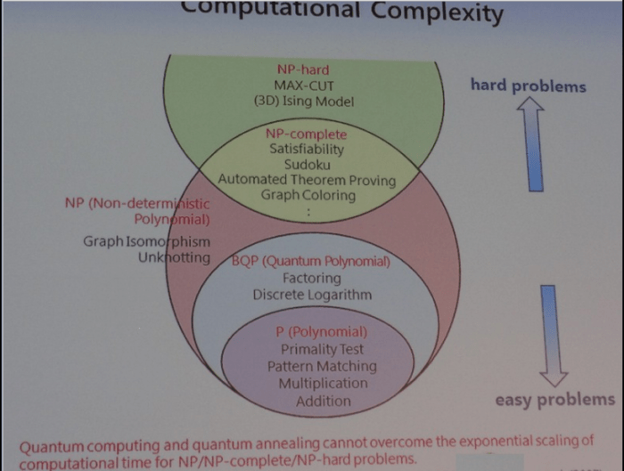
Figure above shows a broad overview of key categories.

_

The class of problems that can be efficiently solved by quantum computers is called BQP, for “bounded error, quantum, polynomial time”. Quantum computers only run probabilistic algorithms, so BQP on quantum computers is the counterpart of BPP (“bounded error, probabilistic, polynomial time”) on classical computers. It is defined as the set of problems solvable with a polynomial-time algorithm, whose probability of error is bounded away from one half. A quantum computer is said to “solve” a problem if, for every instance, its answer will be right with high probability. If that solution runs in polynomial time, then that problem is in BQP.

BQP is contained in the complexity class #P (or more precisely in the associated class of decision problems P#P), which is a subclass of PSPACE. In computational complexity theory, PSPACE is the set of all decision problems that can be solved by a Turing machine using a polynomial amount of space.

_

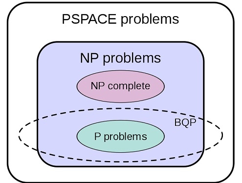
Figure above shows suspected relationship of BQP to other problem spaces.

BQP is suspected to be disjoint from NP-complete and a strict superset of P, but that is not known. Both integer factorization and discrete log are in BQP. Both of these problems are NP problems suspected to be outside BPP, and hence outside P. Both are suspected to not be NP-complete. There is a common misconception that quantum computers can solve NP-complete problems in polynomial time. That is not known to be true, and is generally suspected to be false.

__

Can quantum computers efficiently solve NP-complete problems (such as Traveling Salesman Problem i.e. TSP)?

No.

The class of problems that quantum computers can solve efficiently is called BQP and not NP-complete problem. Having said that, it is important to note that quantum computers may (and do) provide polynomial or constant speed-up in many problems outside BQP (for example, quadratic search speed-up), including such speed-ups for NP-complete problems. For many tasks, even such a moderate speed-up could be of great importance. In cyber security, for example, it affects the size of keys needed to guarantee a requested level of security. We know that it will be hard to solve TSP for huge numbers of cities on a quantum computer — our hardware still has a long way to go before it gets there. But in future, a quantum computer will be able to solve TSP for, let’s say, 50 cities much faster than a regular computer.

Example of BQP problem solved by quantum computer:

When we enter the website of a bank, for example, the communication between us and the bank is encrypted. What is the sophisticated Enigma-like machine that prevents outsiders from hacking into our bank account? Prime numbers. Yes, most of the sensitive communication on the internet is encrypted by a protocol called RSA (standing for the surnames of Ron Rivest, the Israeli Adi Shamir, and Leonard Adelman), whose key is totally public: breaking down a large number into prime numbers. Every computer is capable of hacking RSA, but it would take many years for it to do so. To break down a number of 300 digits into prime numbers would require about 100 years of calculation. A quantum computer would solve the problem within an hour – and hack the internet.  Prime factoring a 300 digit integer is BQP problem.

______

______

Qubit:

Qubits (two-state quantum-mechanical systems) are the basic unit of data in quantum computing. The term “qubit” was coined by Ben Schumacher in a 1993 paper (published in 1995). The paper credits Schumacher’s “intriguing and valuable conversations” with Bill Wootters as the source of the name. The computers that we’re familiar with use bits as their basic unit of data.  Each bit can be either true or false, on or off.  Quantum computers use qubits.  Like bits, qubits can be in one of two states when measured, but that’s where the similarities end. Qubits use quantum mechanical phenomena like superposition and entanglement to exist in multiple states at the same time until measured. Physically, qubits can be any two-level system. For example, the polarization of a photon, or the spin of an electron. Under a strong magnetic field, an electron will polarize with the spin pointing down. Hitting the electron with microwaves will increase its energy and make it spin upward. If the microwave pulse is stopped between positions, the spin is left in a superposition. There is an ensemble qubit which contain a large number of particles that together act as a single qubit and there is what one typically thinks of as a qubit, which is a single particle or material.

Researchers have implemented qubits in several physical representations, including:

1. The spin of atomic nuclei
2. The energy state of an electron suspended by magnetic fields and stimulated by a laser (part of the aptly-named “trapped ion” quantum computer)
3. An electric current which exists in superposition between clockwise and anticlockwise in a superconducting wire.

Mathematicians have developed advanced algorithms that can only be run using quantum computers full of qubits. Algorithms such as Shor’s algorithm for integer factorization (given an integer, find its prime factors) and Grover’s algorithm for searching an unstructured database. These algorithms will be able to solve certain problems much faster than the algorithms our current computers can execute.

_

Two commonly discussed possibilities are the two spin states of an electron:

│1>     and     │0>        as          ↑     and      ↓

or two polarization states of a photon:

│1>     and     │0>      as          H     and      V

The time evolution of a quantum system is usually well approximated by the Schroedinger equation. In a coordinate space representation, for example, the Schroedinger equation is a linear partial differential equation with the property that any linear superposition of eigenfunctions is also a solution. This superposition property of quantum mechanics means that the general state may be written as a superposition of eigenstates. In the case of our 2-state quantum system the general state may be written as:

|ψ〉=α|0〉+β|1〉

According to the standard interpretation of quantum mechanics, any measurement (of spin or polarization) made on this state will always yield one of the two eigenvalues with no way of knowing which one.

_

Qubits are the basic manipulation elements of information in quantum computers. They oppose the bits of classical computing. With them, we move from a deterministic world to a probabilistic world. The following figure compares classical data to quantum data.

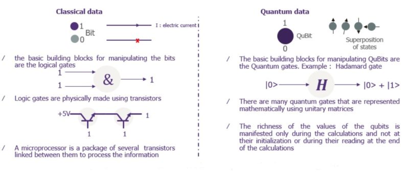
1. |0> and |1> are the notation used to denote states 0 and 1 respectively
2. The main elementary particles of quantum mechanics are: photons and electrons.
3. The most known quantum effects are manifested as: phase of photons, energy level or spin direction of electron.

_

Qubit is the basic unit of quantum information. Due to their unique property called superposition qubits can exist in indeterminate state where we cannot tell if they represent a 0 or a 1, making them exist in both states simultaneously.

To understand it better we have to introduce a definition of Qubit state |ψ〉

It is a unit vector expressed as a linear combination of the basis states. The | 〉 symbol is called a ket and comes from Diracs bra-ket notation, where ket symbolises the quantum state and bra is the complex conjugate of the quantum state:

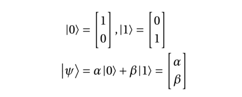
where the coefficients α and β are called the amplitudes of the state. The amplitudes satisfy the following property:

_

Bloch’s Sphere is a mathematical representation of the Qubit:

This model is linked to the representation of the state of a Qubit or of any quantum with two states by a two-dimensional vector whose so-called “norm” length is always 1. The main idea to keep in mind from this mathematical representation is that at any time, except the initialization and the moment of reading, a Qubit can be written as a superposition of two states as the following:

|ψ> = α |0> + β |1>

This vector has the particularity of having two elements: complex numbers α and β.

Remember α² + β² = 1

Remember state |0> sits at the North Pole with α = 1 and β = 0 and state |1> sits at the South Pole with α = 0 and β = 1

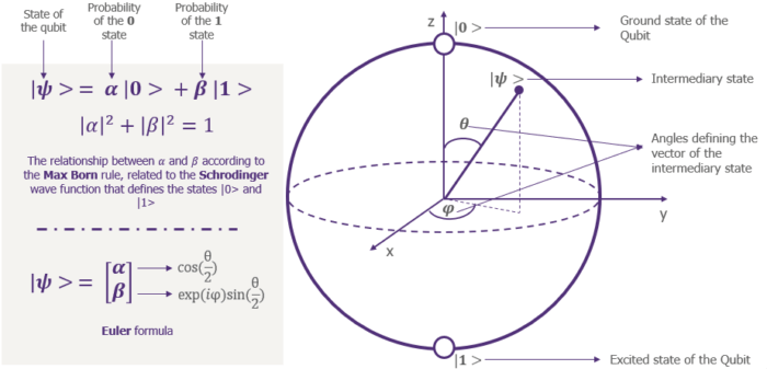
The equivalent formation for a classical computer would just be the two points |0> and |1>, which are shown here as to top and bottom points of the sphere along the z axis.

Note:

The single qubit Bloch sphere provides a useful means of visualizing the state and a neat description of many single qubit operations, enabling physical intuitions and serving as an excellent testbed for ideas about quantum computation and information. However, there is no simple generalization of Bloch sphere for multiple qubits, not even for two qubits.

_

The equation can also be expressed like this:

_

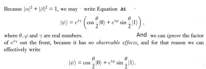
Comparison of Qubits with classical Bits:

A Qubit is the basic unit of quantum information — the quantum version of the classical binary bit physically realised with a two-state device. A Qubit is a two-level quantum-mechanical system. The below figure shows the main differences between a Bit and a Qubit.

_

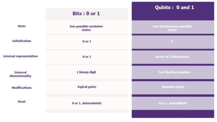
The description of a qubit’s state is a little more complicated with a much wider range of values than a classical bit. To describe the quantum superposition of a qubit requires complex numbers, for example a single qubit’s quantum superposition ψ (a common notation for a superposition, the Greek symbol Psi) could be described as ψ=a|0>+b|1>, where a and b are complex numbers subject to the constraint that |a|²+|b|²=1, with the absolute value of the complex number a squared (|a|²) is equal to the probability that a measurement of the qubit’s state results in the value 0, similarly the absolute value of the complex number b squared (|b|²) is equal to the probability that a measurement of the qubit’s state results in the value 1, and hence the sum of those two probabilities has to sum to 1 (meaning there is exactly a 100% probability of the measured state of a single qubit being either 1 or 0, or using the “bra-ket” notation the states |0> or |1>). Of course we can’t know the actual values of the superposition ψ with a single measurement of a qubit because each measurement will collapse the state to either of the two values under superposition and we lose all of the probabilistic information, but given enough measurements we can attempt to estimate probabilities — or alternatively if we create a known state of ψ prior to a series of transformations through defined quantum gates then we might know the full representation of the resulting state ψ.

_

You may have wondered what the symbols |0⟩ and |1⟩ in the qubit image meant? These are nothing but the notations we use to represent the value of a qubit, and are known as Bra-Ket notations. (|0⟩ +|1⟩)/√2 represents the ‘intermediate’ or superposition value of the qubit, which is a combination of the |0⟩ and |1⟩ state as seen in the figure below:

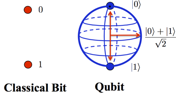
The cool fact about qubits however is that they can take a value of 0 or 1, or both 0 and 1 at the same time! We call this intermediate state as Quantum Superposition. In fact, this is the state every qubit is in, until we decide to measure it because the very act of measuring the value of the qubit makes it ‘collapse’ into one of the two values 0 or 1. We can never see a qubit in its superposition state.

_

If the superposition ψ were to fall exactly on the point |0> at the top of the z axis for instance there would be a 100% probability of a measurement finding a qubit in state 0. Note that the positions of |0> and |1> are arbitrary, if we wanted we could change our basis of measurement and notation to any two points on opposite ends of the sphere. Another common basis besides |0> and |1> are the states |+> and |->, related to our original basis by the formulas |+>=(1/√2)|0>+(1/√2)|1> and |->=(1/√2)|0>-(1/√2)|1>. This +/- basis is notable because both represent a 50% probability of a measurement revealing either 0 or 1 (i.e. |(1/√2)|²=1/2=50%). As we start subjecting a qubit’s superposition to transformation around the Bloch sphere by applying the various quantum gates we may find the alternate measurement and notation basis of |+> and |-> more appropriate, just keep in mind that these notation basis are arbitrary and while it will change the values of a & b to change the basis of notation it won’t change the location on the Bloch sphere. This is worth restating for clarity. When a qubit is subject to transformations by applying a quantum gate, it results in some kind of rotation around the various axis of the Bloch sphere, thus changing the probability of a measurements collapse to states of |0> or |1> (or depending on basis of measurement perhaps another such as |+> or |->). Keep in mind that the Bloch sphere is a two dimensional representation for the state of only a single qubit (this sphere is two dimensional instead of three dimensional because we are restricted to its surface and it is a sphere and not a circle because of the numbers are complex, note that any point on the sphere can be identified with just two variables such as the two angles θ and φ shown in the figure above). As we introduce additional qubits to the system the resulting combined superposition would require a shape of additional dimensions and hence not really as useful for visualization purposes (for example for a two qubit superposition the combined superposition would be described as ψ=a|00>+b|01>+c|10>+d|11>, subject to the restriction that |a|²+|b|²+|c|²+|d|²=1, or in other words |a|² gives the probability that a measurement finds both qubits in the 0 state, |b|² gives the probability of a measurement finding the first qubit in the 0 state and the second qubit in the 1 state, etc.)

_

Often a quantum computer vendor will report on the number of qubits that are achieved as a measure of their scale. As the Hilbert space (dimensionality) of a quantum computer’s state climbs exponentially with the number of qubits as 2^n, this is an important metric. However in evaluating the number of qubits it is important to keep in mind the difference between a functioning logical qubit and a physical qubit. The superimposed state of a physical qubit is extremely fragile, and depending on the architecture, coherence can likely only be maintained for minute fractions of a second, thus there is a demanding need for error correction, comparable to although not identical as the error correction used in a classical computer. These errors cause the ideal shape of the Bloch Sphere to deform in different ways based on the channels of error (i.e. bit flips, phase flips, depolarizing, amplitude dampening, or phase dampening) and their rate. In order to achieve suitable quantum error correction an architecture may have to expend multiple physical qubits to construct a resulting single functioning logical qubit. A key enabler of future more scalable quantum computing architectures will be their ability to maintain their coherence for extended periods and thus reduce the amount of error correction required.

__

You can’t copy a qubit:

A common code pattern in classical programming is copying a value from one variable to another — the second simplest assignment statement (after initializing a variable to a constant), but this action is not supported on qubits due to the no-cloning theorem.

Yes, you can copy a qubit which is neither superimposed nor entangled — it’s in a pure |0> or a pure |1> state, but superimposed or entangled quantum states cannot be copied. In short, you cannot save the arbitrary state of a qubit, nor can you restore the arbitrary state of a qubit. In practice, this restriction can be worked around and is not an insurmountable challenge, but it is one of the more annoying aspects of the quantum computing mindset that takes a bit of getting used to.

__

Multiple Qubits:

What does the combined state of multiple qubits look like?

The combined state of multiple qubits is the tensor product of all the qubits. Below is an example (⊗ is the symbol for the tensor product operation).

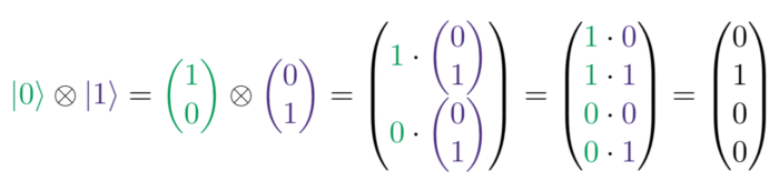
In general, we can tensor product any two matrices by following two steps:

1. Scalar multiply each element in the first matrix by the entire second matrix
2. Combine the resulting matrices according to the original position of their elements

__

Multipartite entanglement?

Current and near-term quantum computers support only bipartite entanglement of qubits — pairs of qubits, but not multipartite entanglement — three or more qubits in a single entanglement. Even with bipartite entanglement, there are severe limits on which pairs of qubits can be entangled and in what direction (which one has to be the control qubit for the CNOT quantum logic gate which creates the entanglement.)  Still it is worth a research effort to at least contemplate whether multipartite entanglement might provide significantly more intellectual leverage for quantum algorithm designers.

__

Qutrits and qudits:

Quantum algorithm designers and quantum programmers will be limited to two-state qubits for the foreseeable future, but there is the potential for more than two states in future quantum computers. A qutrit would have three quantum basis states. A qudit would have ten quantum basis states.

_______

_______

Quantum logic gates and quantum logic circuits:

1. Quantum logic gates are instructions (software), unlike classical logic gates which are hardware:

Historical accident of quantum computing is that instead of focusing on quantum instructions or quantum operations, they decided to call them logic gates, even though a quantum logic gate is not a discrete hardware device like an AND, OR, NOT, XOR, or flip flop in the classical digital logic world of electrical engineers.

Some of the visual tools and diagramming methods for composing quantum programs make it seem as if you are wiring logic devices, when you are simply listing out quantum instructions or operations to be executed sequentially in the order which they are specified. The “wires” are simply a shorthand for referring to the numbering of the qubits (0, 1, 2, …, n).

2. Quantum logic circuits are instruction sequences, not electronic circuits:

When quantum people refer to circuits, once again, they are simply referring to a sequence of instructions of operations to be executed in the sequence written, rather than being “wired” in the same manner as a classical digital logic circuit.

Actually, the execution of a quantum logic circuit is not quite that simple since a significant fraction of the gates (instructions or operations) may be executed in parallel if and when they don’t depend on the results of other gates. Gate execution needs to be scheduled to reflect any dependencies which are implied by the references to qubits and the “wiring” in the individual gates.

The quantum programming language or firmware of the quantum computer will do all the required scheduling and sequencing, driven by the qubit references and “wiring” of the quantum logic circuit.

_

To introduce the quantum gate, let me refer to classical logic gates for comparison. The gate set shown in the figure below represent tool for manipulating bits. The simplest gate, NOT, has a single bit input and the output is the reverse of the original state, i.e. if A was in state 0 then it is transformed to state 1 as an output etc. The other gates shown have an input of two bits and manipulate as a function of the inputs as shown. Note that a gate is considered universal and functionally complete when it is possible to construct all other gate sets using only combinations of that universal gate, as is the case with NAND or NOR gates. With sufficient bits and a set of universal logic gates we have then tools to create any digital circuit.

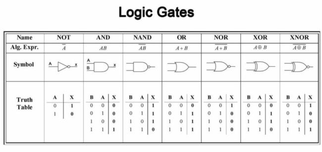
Note that for the most part these common logic gates are irreversible. A logic gate is considered reversible when it is possible to reconstruct the gate’s input bits by inspecting the outputs — thus in order to construct a reversible digital circuit we would need a universal gates with more bits in the output such as the Fredkin or Toffoli gates. All quantum gates are of reversible nature as all quantum gates are unitary matrices.

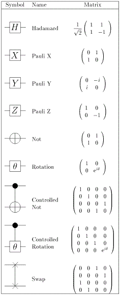
Figure above shows a representative set of quantum gates for universal computation.

There are two types of operations a quantum system can undergo: measurement and quantum state transformations. Most quantum algorithms involve a sequence of quantum state transformations followed by a measurement. For classical computers there are sets of gates that are universal in the sense that any classical computation can be performed using a sequence of these gates. Similarly, there are sets of primitive quantum state transformations, called quantum gates, that are universal for quantum computation.

___

A quantum gate is a unitary matrix:

First of all, quantum gates will be implemented by physical devices, and so they must abide by the laws of quantum physics. One relevant law of physics is that no information is ever lost when transitioning between points in the past and the future. This is known as unitarity. Since our quantum gates define how we transition between states, they too must abide by unitarity.

Secondly, note that our quantum gates will be applied to qubits. We learned earlier that qubits are really just vectors, and so that means quantum gates must somehow operate on vectors. We recall that a matrix is actually just a linear transformation for vectors!

Combining these two ideas, we think of quantum gates as unitary matrices. A unitary matrix is any square matrix of complex numbers such that the conjugate transpose is equal to its inverse. As a quick refresher, the conjugate transpose of a matrix is found by taking the conjugate of each element in the matrix (a + bi → a — bi), and then taking the transpose of the matrix (element ij → element ji). We typically denote the conjugate transpose by the dagger, †.

A key observation about unitary matrices is that they preserve the norm (length of a vector). Suppose we allowed gates that changed the norm, then our qubit’s probabilities may sum to something other than one! That doesn’t make sense since the sum of all probabilities must always be equal to one.

Also notice that, by definition, unitary matrices have an inverse. One implication of this is that we cannot ‘assign’ qubits to arbitrary states. To understand why not, let’s pretend that we did have a quantum gate that could ‘assign’ values, hence, convert any vector of two complex numbers into a specific vector of two complex numbers. This quantum gate would have some underlying representation as a unitary matrix, and that matrix would have an inverse capable of converting a specific vector back into whatever state the qubit was before the operation! But the qubit could have been in any state before the operation and there’s no way to know which! Hence, we cannot ‘assign’ qubits to an arbitrary state. At a higher level, the fact that all quantum gates are invertible is why we often think of quantum computing as a form of reversible computing.

Lastly, notice that because our quantum gates are unitary matrices, they are square by definition, and so our quantum gates must have an equal number of input and output qubits (because square matrices map n standard basis vectors to n columns)! This is quite different from most logic gates; for example, the AND gate takes two inputs and produces one output.

_

Classical computational gates are Boolean logic gates that manipulate information stored in bits. In quantum computing such gates are represented by matrices, and can be visualised as rotations over the Bloch sphere. This visualisation represents the fact that quantum gates are unitary operators, i.e., they preserve the norm of the quantum state (if U is a matrix describing a single qubit gate, then U^†U=I, where U^† is the adjoint of U, obtained by transposing and then complex-conjugating U). In classical computing some gates are “universal”. For example the NAND gate is a gate that evaluates the function “not both A and B” over its two inputs. By stringing together a number of NAND gates it is possible to compute any computable function. Another universal gate is the NOR gate, which evaluates the function “not (A or B)”. In the context of quantum computing it was shown (DiVincenzo 1995) that two-qubit gates (i.e. which transform two qubits) are sufficient to realise a general quantum circuit, in the sense that a circuit composed exclusively from a small set of one- and two-qubit gates can approximate to arbitrary accuracy any unitary transformation of n qubits. Barenco et. al. (1995) showed in particular that any multiple qubit logic gate may be composed in this sense from a combination of single-qubit gates and the two-qubit controlled-not (CNOT) gate, which either flips or preserves its “target” input bit depending on the state of its “control” input bit (specifically: in a CNOT gate the output state of the target qubit is the result of an operation analogous to the classical exclusive-OR (XOR) gate on the inputs). One general feature of quantum gates that distinguishes them from classical gates is that they are always reversible: the inverse of a unitary matrix is also a unitary matrix, and thus a quantum gate can always be inverted by another quantum gate.

_

Unitary gates manipulate information stored in the “quantum register”—a quantum system—and in this sense ordinary (unitary) quantum evolution can be regarded as a computation. In order to read the result of this computation, however, the quantum register must be measured. The measurement gate is a non-unitary gate that “collapses” the quantum superposition in the register onto one of its terms with a probability corresponding to its complex coefficient. Usually this measurement is done in the computational basis but since quantum mechanics allows one to express an arbitrary state as a linear combination of basis states, provided that the states are orthonormal (a condition that ensures normalisation), one can in principle measure the register in any arbitrary orthonormal basis. This, however, doesn’t mean that measurements in different bases are equivalent complexity-wise. Indeed, one of the difficulties in constructing efficient quantum algorithms stems exactly from the fact that measurement collapses the state, and some measurements are much more complicated than others.

_

Quantum algorithms can be described by a quantum circuit when the circuit model is adopted as computational model. A quantum circuit is composed by qubits and gates operating on those qubits. All quantum gates are reversible, unitary operations and are represented by 2ⁿ ×2ⁿ unitary matrices, where n is the number of qubits they act on. The most commonly used gates are single-qubit and two-qubit quantum gates and their corresponding matrix representations.

Another essential operation in quantum circuits is measurement. There are two important properties of this measurement: 1) the act of measuring collapses the quantum state to the state corresponding to the measurement result. 2) this implies that with a single quantum measurement one cannot ‘read’ the superposed qubit state.

Therefore, a quantum state cannot be measured directly without losing the quantum state and thus the stored information.

Finally, it is worth noting that in quantum computing there also exist universal sets of gates and any quantum operation can be approximately implemented by a finite sequence of gates from such a set.

_

Quantum gates transform the state of qubits. For example, the Hadamard gate creates an equal superposition of the two basis states. Without this, what difference would your quantum computer have from a classical computer? In fact, these quantum gates are what make quantum computers so powerful. A quantum computer can process a bunch of classical states in parallel.

For example, let us see a system with 6 qubits.

What a classical computer would do:

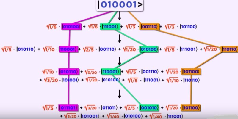
What a quantum computer would do (complete the same problem exponentially faster in just 4 steps even though it’s in the 64th dimensional complex space).

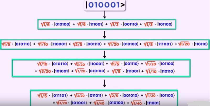
As the number of qubits increase, the number of dimensions increase exponentially! Try to solve a problem involving 50 qubits (that’s 2⁵⁰th dimensional complex space) using a classical computer — it will literally take you forever! Think about all the things you could’ve done during that time.

Quantum computing is incredibly powerful because it does what a classical computer cannot do — solve optimization problems by computing all the possibilities at the same time.

___

A primary and simple example of two entangled qubits is known as the Bell State represented as ψ=(|00>+|11>)/√2, where using the same derivation of probability we find that there is a 50% probability of both qubits being found in the 0 state, a 50% chance of both qubits being found in the 1 state, and a 0% probability of the qubits being found in opposite states such as |01> or |10>. One way to prepare a Bell state is to take two qubits both initialized to |0>, then apply a Hadamard gate to one and CNOT gate. Once we achieve the Bell State, if we measure one of the two qubits we will immediately know the state of the other.

Just like in a classical computer, there exists a set of quantum gates that allow us to simulate any reversible quantum circuit aka a universal quantum gate set. This gate set can be achieved with the CNOT and single qubit unitary gates, or alternatively with multi qubit gates such as a quantum analog to the Fredkin gate.

___

Quantum circuits:

A quantum circuit (also called quantum network or quantum gate array) generalizes the idea of classical circuit families, replacing the AND, OR, and NOT gates by elementary quantum gates. A quantum gate is a unitary transformation on a small (usually 1, 2, or 3) number of qubits. The main 2-qubit gate we have seen is the controlled-NOT (CNOT) gate. Adding another control register, we get the 3-qubit Toffoli gate, also called controlled-controllednot (CCNOT) gate. This negates the third bit of its input if both of the first two bits are 1. The Toffoli gate is important because it is complete for classical reversible computation: any classical computation can be implemented by a circuit of Toffoli gates. This is easy to see: using auxiliary wires with fixed values, Toffoli can implement AND (fix the 3rd ingoing wire to 0) and NOT (fix the 1st and 2nd ingoing wire to 1). It is known that AND and NOT-gates together suffice to implement any classical Boolean circuit, so if we can apply (or simulate) Toffoli gates, we can implement any classical computation in a reversible manner.

Mathematically, such elementary quantum gates can be composed into bigger unitary operations by taking tensor products (if gates are applied in parallel to different parts of the register), and ordinary matrix products (if gates are applied sequentially). We have already seen a simple example of such a circuit of elementary gates in the previous chapter, namely to implement teleportation.

The basic memory component in classical computing is a bit, which can be in two states, “0” or “1”. A computer (or circuit) has 𝑛 bits, and it can perform certain logical operations on them. The NOT gate, acting on a single bit, and the AND gate, acting on two bits, suffice for universal classical computing. This means that a computation based on another collection of logical gates, each acting on a bounded number of bits, can be replaced by a computation based only on NOT and AND. Classical circuits equipped with random bits lead to randomized algorithms, which are both practically useful and theoretically important.

Quantum computers (or circuits) allow the creation of probability distributions that are well beyond the reach of classical computers with access to random bits. A qubit is a piece of quantum memory. The state of a qubit can be described by a unit vector in a two dimensional complex Hilbert space 𝐻. For example, a basis for 𝐻 can correspond to two energy levels of the hydrogen atom or to horizontal and vertical polarizations of a photon. Quantum mechanics allows the qubit to be in a superposition of the basis vectors, described by an arbitrary unit vector in 𝐻. The memory of a quantum computer consists of 𝑛 qubits. Let 𝐻𝑘 be the two-dimensional Hilbert space associated with the 𝑘th qubit. The state of the entire memory of 𝑛 qubits is described by a unit vector in the tensor product 𝐻1 ⊗ 𝐻2 ⊗ ⋯ ⊗ 𝐻𝑛. We can put one or two qubits through gates representing unitary transformations acting on the corresponding two- or four-dimensional Hilbert spaces, and as for classical computers, there is a small list of gates sufficient for universal quantum computing. Each step in the computation process consists of applying a unitary transformation on the large 2^𝑛-dimensional Hilbert space, namely, applying a gate on one or two qubits, tensored with the identity transformation on all other qubits. At the end of the computation process, the state of the entire computer can be measured, giving a probability distribution on 0–1 vectors of length 𝑛.

A few words on the connection between the mathematical model of quantum circuits and quantum physics: In quantum physics, states and their evolutions (the way they change in time) are governed by the Schrödinger equation. A solution of the Schrödinger equation can be described as a unitary process on a Hilbert space, and quantum computing processes as we just described form a large class of such quantum evolutions.

_

Quantum registers vs classical registers:

Registers are a type of computer memory used to quickly accept, store, and transfer data and instructions that are being used immediately by the CPU. … A processor register may hold an instruction, a storage address, or any data (such as bit sequence or individual characters).

A register is a temporary storage area built into a CPU. Some registers are used internally and cannot be accessed outside the processor, while others are user-accessible. Most modern CPU architectures include both types of registers.

Registers vary in both number and size, depending on the CPU architecture. Some processors have 8 registers while others have 16, 32, or more. For many years, registers were 32-bit, but now many are 64-bit in size. A 64-bit register is necessary for a 64-bit processor, since it enables the CPU to access 64-bit memory addresses. A 64-bit register can also store 64-bit instructions, which cannot be loaded into a 32-bit register. Therefore, most programs written for 32-bit processors can run on 64-bit computers, while 64-bit programs are not backwards compatible with 32-bit machines.

Here is an example using a register of 4 Qubits:

_

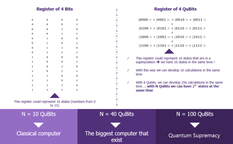
The table below gives a detailed overview of a register of n Qubits compared to a register of n bits.

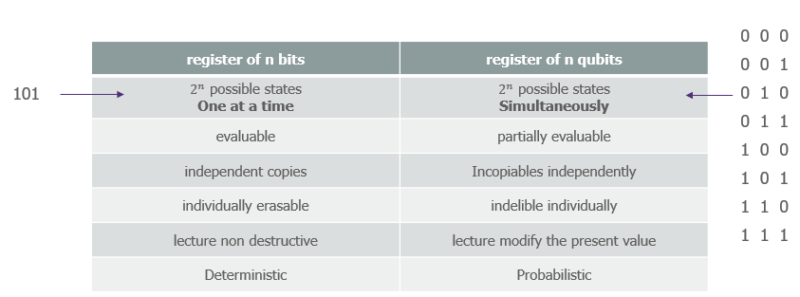
These 2 of power n states, however, do not really correspond to a capacity of information storage. It is a state superposition capability that is then applied to treatments to highlight the combinations that we search according to an algorithm given.

_____

Global architecture of a quantum computer:

_____

_____

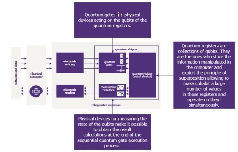
Quantum Computation Algorithms:

_

Algorithms and code are not the same thing:

Loosely speaking, a lot of people, including otherwise competent professionals, will treat algorithms and code as being the same thing, but it simply isn’t true.

An algorithm is a series of steps for solving a problem, completing a task or performing a calculation. In mathematics and computer science, an algorithm is a finite sequence of well-defined, computer-implementable instructions, typically to solve a class of problems or to perform a computation.

An algorithm is more of a higher-level specification of how the desired function or purpose is achieved, at a higher level, rather than at the level of raw code. It may have relatively detailed steps, but not as detailed as is required to actually be directly translated into machine language for a computer, classical or quantum.

Code on the other hand is in fact detailed enough that it can be directly and 100% translated into executable machine language instructions. Code is always expressed in a programming language and then compiled into executable code or an intermediate form which can be interpreted as if it had been compiled into executable code.

Algorithms may sometimes be expressed in a form that superficially looks like code or at least a code-like language, but generally they are expressed in more expressive forms of language.

Code is often low complexity, repetitive or non-critical. For example, code that displays a user interface, validates input, performs a transaction or calculates a value is usually straightforward to implement. Algorithms are at another level of complexity and may begin life as a research project or similarly intensive effort. Any code that is composed by a developer on the fly that doesn’t solve a big problem isn’t typically considered an algorithm.

It should be noted that it is common for firms to use the term algorithm simply because it sounds good. As such, the term is beginning to lose its meaning and is becoming increasingly synonymous with code.

_

Evolution vs. iteration:

Classical algorithms and classical code are based in large part on the concept of iteration — sequencing though lists of items and lists of alternatives. That may be great for classical computers, but just doesn’t fit in with the quantum world. The heart of the quantum world is evolution. All items are evolving in parallel. There is still sequencing in the quantum world, but it is time sequencing or time evolution, with all items qubits evolving in parallel, at the same time. This is a major change in mindset for people coming from the classical world. Although, it is not so different from the world of distributed computing, where each computer system is operating completely in parallel with all other computer systems. That’s true, but people struggle immensely trying to get distributed systems to function properly.

In summary, step one in contemplating a quantum algorithm is how exactly you expect all of the elements of the quantum computation to be evolving in parallel, interacting (entangling) as needed. Quantum computing still has iteration, but it is iterating through time, all items in parallel, rather than iterating item by item.

_

In quantum computing, a quantum algorithm is an algorithm which runs on a realistic model of quantum computation, the most commonly used model being the quantum circuit model of computation. A classical (or non-quantum) algorithm is a finite sequence of instructions, or a step-by-step procedure for solving a problem, where each step or instruction can be performed on a classical computer. Similarly, a quantum algorithm is a step-by-step procedure, where each of the steps can be performed on a quantum computer. Although all classical algorithms can also be performed on a quantum computer, the term quantum algorithm is usually used for those algorithms which seem inherently quantum, or use some essential feature of quantum computation such as quantum superposition or quantum entanglement.

Problems which are undecidable using classical computers remain undecidable using quantum computers. What makes quantum algorithms interesting is that they might be able to solve some problems faster than classical algorithms because the quantum superposition and quantum entanglement that quantum algorithms exploit probably can’t be efficiently simulated on classical computers.

_

Algorithm design is a highly complicated task, and in quantum computing, delicately leveraging the features of quantum mechanics in order to make our algorithms more efficient makes the task even more complicated. Let us first convince ourselves that quantum computers can be harnessed to perform standard, classical, computation without any computational speed-up. In some sense this is obvious, given the belief in the universal character of quantum mechanics, and the observation that any quantum computation that is diagonal in the computational basis, i.e., that involves no interference between the qubits, is effectively classical. Yet the demonstration that quantum circuits can be used to simulate classical circuits is not straightforward (recall that the former are always reversible while the latter use gates which are in general irreversible). Indeed, quantum circuits cannot be used directly to simulate classical computation, but the latter can still be simulated on a quantum computer using an intermediate gate, namely the Toffoli gate. This universal classical gate has three input bits and three output bits. Two of the input bits are control bits, unaffected by the action of the gate. The third input bit is a target bit that is flipped if both control bits are set to 1, and otherwise is left alone. This gate is reversible (its inverse is itself), and by stringing a number of such gates together one can simulate any classical irreversible circuit. Consequently, using the quantum version of the Toffoli gate (which by definition permutes the computational basis states similarly to the classical Toffoli gate) one can simulate, although rather tediously, irreversible classical logic gates with quantum reversible ones. Quantum computers are thus capable of performing any computation which a classical deterministic computer can do.

What about probabilistic computation? Not surprisingly, a quantum computer can also simulate this type of computation by using another famous quantum gate, namely the Hadamard gate, a single-qubit gate which receives as input the state |0⟩ and produces the state |0⟩+|1⟩/√2. Measuring this output state yields |0⟩ or |1⟩ with 50/50 probability, which can be used to simulate a fair coin toss.

Obviously, if quantum algorithms could be used only to simulate classical algorithms, then the technological advancement in information storage and manipulation, encapsulated in “Moore’s law”, would have only trivial consequences on computational complexity theory, leaving the latter unaffected by the physical world. But while some computational problems will always resist quantum “speed-up” (in these problems the computation time depends on the input, and this feature will lead to a violation of unitarity hence to an effectively classical computation even on a quantum computer—see Myers (1997) and Linden and Popescu (1998)), the hope is, nonetheless, that quantum algorithms may not only simulate classical ones, but that they will actually outperform the latter in some cases, and in so doing help to re-define the abstract notions of tractability and intractability and violate the physical Church-Turing thesis, at least as far as computational complexity is concerned.

_

The big classes of quantum algorithms:

1. Search algorithms: search algorithms based on those of Deutsch-Jozsa, Simon and Grover.
2. Algorithms that seek a balance point of a complex system: algorithms that seek a balance point of a complex system like in the training of neural networks, the search for an optimal path in networks or process optimization.
3. Algorithms based on Quantum Fourier Transforms (QFT) : such as Shor’s Integer Factorization, which triggered a debate between people who are wanting to create quantum computers capable of breaking public RSA-type security keys, and people being the ones looking for to protect digital communications with algorithms resistant to the fast factorization of integers.
4. Simulation algorithms of quantum mechanisms: which serve in particular to simulate interactions between atoms in various molecular structures, inorganic and organic.

_

Reduction of the wave packet: reduces the power of acceleration on some classical algorithms:

The reduction of the wave packet is a fundamental notion of quantum mechanics and thus of quantum computing that, after a measurement, a physical system sees its state completely reduced to the one that has been measured. This notion of wave packet reduction involves many difficulties on the implementation plane of quantum algorithms, and more particularly the parallelization of intermediate computations, which is the main gain of the quantum. Concretely, to be able to implement a classical algorithm on a quantum computer it is necessary to find an implementation which takes advantage of the power of the parallelisation only in the intermediate calculations and giving only one result.

_

Developing new quantum algorithms is an active field of research that has seen increasing growth in the past couple of years. Many companies and research institutes are trying to come up with new quantum algorithms that solve relevant computational problems better than classical algorithms. The main quantum algorithms developed so far are:

1. Shor’s algorithm: factorization of large numbers and solving the discrete logarithm problem. This algorithm has the potential to break most of the currently used public-key cryptography.

Shor’s algorithm exploits the ingenious number theoretic argument that two prime factors p, q of a positive integer N = pq can be found by determining the period of a function f(x)=yxmodN, for any y<N which has no common factors with N other than 1 (Nielsen and Chuang 2000). The period r of f(x) depends on y and N. Once one knows it, one can factor N if r is even and yr2≠−1 mod N, which will be jointly the case with probability greater than 12 for any y chosen randomly (if not, one chooses another value of y and tries again). The factors of N are the greatest common divisors of yr2±1 and N, which can be found in polynomial time using the well-known Euclidean algorithm. In other words, Shor’s remarkable result rests on the discovery that the problem of factoring reduces to the problem of finding the period of a certain periodic function f:Zn→ZN, where Zn is the additive group of integers mod n (Note that f(x)=yx mod N so that f(x+r)=f(x) if x+r≤n. The function is periodic if r divides n exactly, otherwise it is almost periodic). That this problem can be solved efficiently by a quantum computer is hinted at by Simon’s algorithm, which considers the more restricted case of functions periodic under bit-wise modulo-2 addition as opposed to the periodic functions under ordinary addition considered here.

Shor’s result is the most dramatic example so far of quantum “speed-up” of computation, notwithstanding the fact that factoring is believed to be only in NP and not in NP-complete. To verify whether n is prime takes a number of steps which is a polynomial in log2n (the binary encoding of a natural number n requires log2n resources). But nobody knows how to factor numbers into primes in polynomial time, and the best classical algorithms we have for this problem are sub-exponential. This is yet another open problem in the theory of computational complexity. Modern cryptography and Internet security protocols are based on these facts (Giblin 1993): It is easy to find large prime numbers fast, and it is hard to factor large composite numbers in any reasonable amount of time. The discovery that quantum computers can solve factoring in polynomial time has had, therefore, a dramatic effect. The implementation of the algorithm on a physical machine would have economic, as well as scientific consequences (Alléaume et al. 2014).

2. Grover’s algorithm: searching in an unsorted list. This is a generic method that can be applied to many types of computational problems. Quantum computers offer polynomial speedup for some problems. The most well-known example of this is quantum database search, which can be solved by Grover’s algorithm using quadratically fewer queries to the database than that are required by classical algorithms. In this case, the advantage is not only provable but also optimal, it has been shown that Grover’s algorithm gives the maximal possible probability of finding the desired element for any number of oracle lookups. Several other examples of provable quantum speedups for query problems have subsequently been discovered, such as for finding collisions in two-to-one functions and evaluating NAND trees.

The running time of Grover’s algorithm on a quantum computer will scale as the square root of the number of inputs (or elements in the database), as opposed to the linear scaling of classical algorithms. A general class of problems to which Grover’s algorithm can be applied is Boolean satisfiability problem. In this instance, the database through which the algorithm is iterating is that of all possible answers. An example (and possible) application of this is a password cracker that attempts to guess the password or secret key for an encrypted file or system. Symmetric ciphers such as Triple DES and AES are particularly vulnerable to this kind of attack.

3. Quantum Approximate Optimization Algorithm (QAOA): A general method to solve optimization problems under specific conditions. Many problems in finance, manufacturing, transport etc. can be formulated as an optimization problem, which shows the potential impact of this algorithm.
4. Harrow Hassidim Lloyd (HHL) algorithm: This algorithm solves a linear system of equations. As linear systems are in the core of many science and engineering problems, the potential speedup presented by the HHL algorithm can have a major impact.

An important parameter to the success of a quantum algorithm is its performance compared to classical algorithms. From a theoretical point of view there are certain computational problems that are proven to be intractable with classical computers (or at least infeasible within a reasonable time). An implementation of a quantum algorithm that solves such a problem would be a great achievement. On a more practical level, a quantum algorithm will already be extremely successful if it performs better than a classical algorithm.

This creates a (healthy) competition between classical and quantum algorithm designers. Interesting examples of this competition are recent implementations of QAOA and HHL that seemed to outperform the best known classical algorithms. This success was of very limited duration as new classical algorithms were soon developed that perform even better. The bottom line is: even before the first demonstration of a quantum computer, the progress in this field is having a positive effect on the field in general.

_

Need for libraries of quantum code:

Countless libraries of functions, classes, modules, frameworks, and sample programs abound for classical computing, so that starting a new project doesn’t mean having to start from scratch. Granted, it will take some time to compete with the vast code libraries accumulated over 80 years of classical computing, but the need is clear. Open source and project and source code repositories such as GitHub will facilitate the process. Even over 40 years ago, Microsoft was able to get a head start on their microcomputer tools using software readily available on magnetic tape from the Digital Equipment Corporation User Society (DECUS). There already is a modest amount of quantum example code on GitHub today, but we’re still in only the very early days. And a lot of it is simply examples and very fragmentary rather than being ready to incorporate into realistic programs. The fact that the quantum world doesn’t have rich code structuring tools such as compiled functions, classes, modules, and formal libraries, greatly impedes code sharing at any more than the level of example stand alone programs.

__

The Quantum Computing Programming Language:

Quantum algorithms provide the ability to analyze the data and offer simulations based on the data. These algorithms are written in a quantum-focused programming language. Several quantum languages have been developed by researchers and technology companies.

These are a few of the quantum computing programming languages:

1. QISKit: The Quantum Information Software Kit from IBM is a full-stack library to write, simulate, and run quantum programs.
2. Q#: The programming language included in the Microsoft Quantum Development Kit. The development kit includes a quantum simulator and algorithm libraries.
3. Cirq: A quantum language developed by Google that uses a python library to write circuits and run these circuits in quantum computers and simulators.
4. Forest: A developer environment created by Rigetti Computing that is used to write and run quantum programs.

______

______

Quantum operations:

In this article, “quantum computing” has so far been used as a blanket term describing all computations that utilize quantum phenomena. There are actually multiple types of operational frameworks. Logical, gate-based quantum computing is probably the best recognized. In it, qubits are prepared in initial states and then subject to a series of “gate operations,” like current or laser pulses depending on qubit type. Through these gates the qubits are put in superpositions, entangled, and subjected to logic operations like the AND, OR, and NOT gates of traditional computation. The qubits are then measured and a result obtained.

Another framework is measurement-based computation, in which highly entangled qubits serve as the starting point. Then, instead of performing manipulation operations on qubits, single qubit measurements are performed, leaving the targeted single qubit in a definitive state. Based on the result, further measurements are carried out on other qubits and eventually an answer is reached.

A third framework is topological computation, in which qubits and operations are based on quasiparticles and their braiding operations. While nascent implementations of the components of topological quantum computers have yet to be demonstrated, the approach is attractive because these systems are theoretically protected against noise, which destroys the coherence of other qubits.

Finally, there are the analog quantum computers or quantum simulators envisioned by Feynman. Quantum simulators can be thought of as special purpose quantum computers that can be programmed to model quantum systems. With this ability they can target questions such as how high-temperature superconductors work, or how certain chemicals react, or how to design materials with certain properties.

_

How does a quantum computer work?

Having laid the groundwork of building blocks for computation such as qubits, error correction, gates, and entanglement, I think we’re finally ready to dive into the actual operation of a quantum computation. It’s actually pretty simple:

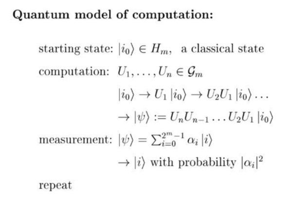
A quantum computation starts with initialized qubits, and then a series of unitary transformations are applied to transform the system into the desired configuration of superposition and entanglement — these series of gates are how we actualize a quantum algorithm. Once the series of gates and transformations are applied measurements are taken of the qubits. An important distinction between quantum and classical computers is that a quantum computer is probabilistic, thus these measurements of algorithmic outputs only give the proper solution within an algorithm specific confidence interval. The computation is then repeated until satisfactory probable certainty of solution can be achieved.

__

Measuring a qubit:

Suppose a (hypothetical!) quantum physicist named Alice prepares a qubit in her laboratory, in a quantum state α∣0⟩+β∣1⟩. Then she gives her qubit to another quantum physicist, Bob, but doesn’t tell him the values of α and β. Is there some way Bob can figure out α and β? That is, is there some experiment Bob can do to figure out the identity of the quantum state?

The surprising answer to this question turns out to be NO! There is, in fact, no way to figure out α and β if they start out unknown. To put it a slightly different way, the quantum state of any system – whether it be a qubit or a some other system – is not directly observable.

Similarly, when you first start learning about quantum circuits, it seems like we should be able to observe the amplitudes of a quantum state whenever we like. But that turns out to be prohibited by the laws of physics. Those amplitudes are better thought of as a kind of hidden information.

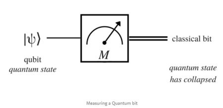
We have a qubit (a superposed quantum state) formed by some linear combination of |0> and |1>. After measurement, it becomes a classical bit (0 or 1).

Two very simple examples to illustrate this point:

1. Measurements destroy the quantum state in most cases.
2. Energy enters and leaves the system.

So, what can we figure out from the quantum state? Rather than somehow measuring α and β, there are other ways of getting useful information out of a qubit. Let me describe an especially important process called measurement in the computational basis. This is a fundamental primitive in quantum computing: it’s the way we typically extract information from our quantum computers. I’ll explain now how it works for a single qubit, and later generalize to multi-qubit systems.

Suppose a qubit is in the state α∣0⟩+β∣1⟩. When you measure this qubit in the computational basis it gives you a classical bit of information: it gives you the outcome 0 with probability ∣α∣^2, and the outcome 1 with probability ∣β∣^2.

To think a little more concretely about this process, suppose your qubit is instantiated in some physical system. Perhaps it’s being stored in the state of an atom somehow. It doesn’t matter exactly what, but you have this qubit in your laboratory. And you have some measurement apparatus, probably something large and complicated, maybe involving lasers and microprocessors and a screen for readout of the measurement result. And this measurement apparatus interacts in some way with your qubit.

After the measurement interaction, your measurement apparatus registers an outcome. For instance, it might be that you get the outcome 0. Or maybe instead you get the outcome 1. The crucial fact is that the outcome is ordinary classical information – the stuff you already know how to think about – which you can then use to do other things, and to control other processes.

So the way a quantum computation works is that we manipulate a quantum state using a series of quantum gates, and then at the end of the computation (typically) we do a measurement to read out the result of the computation. If our quantum computer is just a single qubit, then that result will be a single classical bit. If, as is more usually the case, it’s multiple qubits, then the measurement result will be multiple classical bits.

A fundamental fact about this measurement process is that it disturbs the state of the quantum system. In particular, it doesn’t just leave the quantum state alone. After the measurement, if you get the outcome 0 then the state of the qubit afterwards (the “posterior state”) is the computational basis state ∣0⟩. On the other hand, if you get the outcome 1 then the posterior state of the qubit is the computational basis state ∣1⟩.

Summing all this up: if we measure a qubit with state α∣0⟩+β∣1⟩ in the computational basis, then the outcome is a classical bit: either 0, with probability ∣α∣|^2 or 1, with probability ∣β∣^2. The corresponding state of the qubit after the measurement is ∣0⟩| or ∣1⟩.

A key point to note is that after the measurement, no matter what the outcome, complex numbers α and β are gone. No matter whether the posterior state is ∣0⟩ or ∣1⟩, there is no trace of α or β. And so you can’t get any more information about them. A complex number is a number that can be expressed in the form a + bi, where a and b are real numbers, and i is a solution of the equation x² = −1. Because no real number satisfies this equation, i is called an imaginary number.

One reason this is important is because it means you can’t store an infinite amount of classical information in a qubit. After all, α is a complex number, and you could imagine storing lots of classical bits in the binary expansion of the real component of α. If there was some experimental way you could measure the value of α exactly, then you could extract that classical information. But without a way of measuring α that’s not possible. Besides measurement in the computational basis, there are other types of measurement you can do in quantum systems. But there’s a sense in which computational basis measurements turn out to be fundamental. The reason is that by combining computational basis measurements with quantum gates like the Hadamard and NOT (and other) gates, it’s possible to simulate arbitrary quantum measurements. So this is all you absolutely need to know about measurement, from an in-principle point of view.

_

Applications on quantum computers:

Code is of course essential for software and applications, and algorithms are essential for code, but algorithms alone and even code alone do not constitute an application, and it is applications which justify the expense and effort of advanced computers.

The missing pieces needed for applications which are not found on quantum computers include:

1. Data. It lives somewhere and comes from somewhere, but not on the quantum computer itself.
2. User interaction and user experience. Again, this happens on classical computers, not the quantum computer.
3. Algebraic computation. Maybe someday quantum computers will support this, but not soon.
4. Complex control flow. Requires the hybrid mode of operation.
5. Complex data structures. Ditto.
6. Transforming real data to and from the form of data that exists on a quantum computer — qubits in the |0> and |1> quantum states. All of this must be performed on a classical computer.
7. Networking and distributed computing. Outside the realm of quantum computing. Someday there may be forms of quantum networking, but not soon.

In short, a quantum application is a lot more than quantum computation on a quantum computer.

__

Hybrid mode of operation:

The most prevalent way of doing quantum computing today, arguably, is called hybrid classical-quantum computing. The idea is simple — there are some things that classical computers can do extremely well and there are certain things that quantum computers can do extremely well. Both of them also have their own limitations. So why not leverage the best in those two types of hardware? Not all problems will be able to be completely solved by a discrete quantum program. Instead, the original problem may need to be broken into a sequence of smaller problems — partitioned into chunks, each of which can be processed by its own quantum circuit or quantum program, and then a classical computer program can integrate the individual results from each of those smaller problems. That’s the simplest form of the hybrid mode of operation — a simple, linear, multi-step sequence.

The next level of complexity is conditional execution, which quantum computers do not support. Instead, the classical program sends shorter quantum circuits to calculate intermediate results, which the classical program retrieves and then makes a decision about what alternative quantum circuits should be conditionally executed.

Iteration can be added as well in a similar manner, with the classical program examining the intermediate quantum results and then deciding whether and how to re-execute that same quantum circuit. In fact, conditional and iterative execution quantum circuits can be combined in any arrangement, such as nested iterations or conditional execution within an iteration.

The only downside is that the measurement process which is needed to obtain intermediate results has the downside of what is called collapse of the wave function, where any quantum state of superposition or entanglement of a qubit vanishes when that qubit is measured. It doesn’t completely vanish, but it collapses to one of the two basis states, |0> or |1>, based on the probability computed and maintained for each basis state as the qubit evolves as each successive quantum logic gate of the logic circuit is executed. The qubit is then 100% in the measured state, the one into which it collapsed. It will vary from program to program whether the loss of quantum state for superposition and entanglement is a big deal, a major annoyance, a minor annoyance, or not a problem at all. It could be that the quantum state for that particular circuit is no longer needed.

In an iteration, it could be that each iteration needs to do a different form of preparation anyway.

In conditional execution, it will vary whether the previous quantum state is needed for the conditional logic circuit. It may not be needed at all, or if it is needed, the previous circuit could simply be re-executed, but without state-collapsing measurement, followed by the conditional logic circuit — all as one, contiguous circuit.

Even if there are a number of conditional branches in a sequence, each branch can simply begin with as much of the preceding circuits as needed to reconstruct any needed quantum state, if it is needed at all.

The intermediate results may literally be intermediate and thrown away after being examined by the classical program, or they may be incremental final results, to be accumulated and saved or processed when the program finishes all of its quantum processing. Or, that saving and processing may be done incrementally as well.

The hybrid mode of operation works for quantum simulators as well as real quantum computers.

__

Hybrid algorithms, a 2019 study:

In recent years, quantum devices have become available that enable researchers — for the first time — to use real quantum hardware to begin to solve scientific problems. However, in the near term, the number and quality of qubits (the basic unit of quantum information) for quantum computers are expected to remain limited, making it difficult to use these machines for practical applications.

A hybrid quantum and classical approach may be the answer to tackling this problem with existing quantum hardware. Researchers at the U.S. Department of Energy’s (DOE) Argonne National Laboratory and Los Alamos National Laboratory, along with researchers at Clemson University and Fujitsu Laboratories of America, have developed hybrid algorithms to run on quantum machines and have demonstrated them for practical applications using IBM quantum computers and a D-Wave quantum computer.

The team’s work is presented in an article entitled “A Hybrid Approach for Solving Optimization Problems on Small Quantum Computers” that appears in the June 2019 issue of the Institute of Electrical and Electronics Engineers (IEEE) Computer Magazine.

Concerns about qubit connectivity, high noise levels, the effort required to correct errors, and the scalability of quantum hardware have limited researchers’ ability to deliver the solutions that future quantum computing promises.

The hybrid algorithms that the team developed employ the best features and capabilities of both classical and quantum computers to address these limitations. For example, classical computers have large memories capable of storing huge datasets — a challenge for quantum devices that have only a small number of qubits. On the other hand, quantum algorithms perform better for certain problems than classical algorithms.

To distinguish between the types of computation performed on two completely different types of hardware, the team referred to the classical and quantum stages of hybrid algorithms as central processing units (CPUs) for classical computers and quantum processing units (QPUs) for quantum computers.

The team seized on graph partitioning and clustering as examples of practical and important optimization problems that can already be solved using quantum computers: a small graph problem can be solved directly on a QPU, while larger graph problems require hybrid quantum-classical approaches.

As a problem became too large to run directly on quantum computers, the researchers used decomposition methods to break the problem down into smaller pieces that the QPU could manage — an idea they borrowed from high-performance computing and classical numerical methods. All the pieces were then assembled into a final solution on the CPU, which not only found better parameters, but also identified the best sub-problem size to solve on a quantum computer.

Such hybrid approaches are not a silver bullet; they do not allow for quantum speedup because using decomposition schemes limits speed as the size of the problem increases. In the next 10 years, though, expected improvements in qubits (quality, count, and connectivity), error correction, and quantum algorithms will decrease runtime and enable more advanced computation.

In the meantime this approach will enable researchers to use near-term quantum computers to solve applications that support the DOE mission. For example, it can be applied to find community structures in metabolic networks or a microbiome.

__

Issues of scalability:

In theory, a solution to a problem on a quantum computer should be much more scalable than a comparable solution on a classical computer. That’s the theory. But in practice, scalability is more of an art and craft than a true science. Realizing the potential for scalability of quantum computers is a major challenge, and in many cases not even achievable, at least in the relatively near future. Even if the hardware is indeed scalable, that does not guarantee the same for algorithms. There are likely to be lots of practical issues, beyond the basic theory.

Connectivity of qubits is likely to be a real issue. Or rather the significant restrictions on connectivity on current quantum computers is an issue. Connectivity may not grow at the same rate as qubit count grows. And even when connectivity does increase, it doesn’t keep up with the raw number of quantum states which those qubits support. A 10-qubit quantum computer supports 1,024 quantum states, but only five concurrent entangled pairs of qubits, and not all combinations of pairs. A 20-qubit quantum computer supports a million quantum states, but only ten concurrent entangled pairs of qubits, and not all combinations of pairs. So, algorithms must use entanglement very sparingly, which limits scalability. Shor’s algorithm was billed as killing public-key encryption, but once again, an algorithm which works very well with a small amount of data simply doesn’t scale.

One unexplored area of scalability is that current quantum logic gates are individual operations on individual qubits, or pairs of qubits, or occasionally three qubits, but as the number of qubits used by an algorithm rises dramatically, that means that many quantum logic gates must be executed, some sequentially, but potentially many in parallel. The qubits may operate in parallel, but the firmware code and digital logic that sequences through the gates is classical, not quantum, so it does not operate fully in parallel, which raises the prospect that there may be a limit to how many qubits can be operated on in parallel before the coherence limit is reached. The documentation for each machine needs to specify how many gates can operate in parallel, and if there are any limits. This is not an issue with small numbers of qubits, but once we get dozens and then hundreds, and eventually thousands, this matter must be addressed more directly.

The hybrid mode of operation also presents scalability challenges if the classical code needs to execute for longer than the coherence time of the qubits. But that begs the question of the degree to which the quantum computer permits the classical code to interrupt the flow of quantum logic gates, measure some qubits and leave others live, go off and do some classical computation, and then resume gate execution while keeping the unmeasured gates alive. That may not be so practical today on some machines, but will probably be important in the longer run, especially as the size and complexity of qubit count and gate count rise dramatically. Otherwise, the classical code will be forced to completely restart the quantum program from the start, which isn’t a problem for smaller qubit and gate counts, but could be problematic for higher qubit and gate counts.

Scalability is nothing new in computing, but a wide variety of tricks and techniques have been developed over the decades to allow an interesting level of scaling on classical computers. Unfortunately, most of those efforts are simply not relevant to the much more austere programming model of a quantum computer. For example, numerous approaches to indexing of data for databases and search engines.

Much more research is needed on scalability of both hardware and algorithms. Meanwhile, designers of quantum algorithms will need to invest an extraordinary level of effort to achieve even a modest degree of scaling.

______

______

Overview of building quantum computer:

_

Quantum hardware:

In classical computers, bits correspond to voltage levels in silicon circuits. Quantum computing hardware can be implemented by many different physical realizations of qubits: trapped ions, superconducting, neutral atoms, electron spin, light polarization, topological qubits. Quantum hardware is an emergent technology. Qubits are fragile by nature and become less coherent as they interact with their environment. Balancing fidelity of the system with scalability is needed. The larger the scale (that is, number of qubits), the higher the error rate.

_

Building Quantum Computers is Hard:

We have decades of experience building ordinary, transistor-based computers with conventional architectures; building quantum machines means reinventing the whole idea of a computer from the bottom up. First, there are the practical difficulties of making qubits, controlling them very precisely, and having enough of them to do really useful things. Next, there’s a major difficulty with errors inherent in a quantum system—”noise” as this is technically called—which seriously compromises any calculations a quantum computer might make. There are ways around this (“quantum error correction”), but they introduce a great deal more complexity. There’s also the fundamental issue of how you get data in and out of a quantum computer, which is, itself, a complex computing problem. Some critics believe these issues are insurmountable; others acknowledge the problems but argue the mission is too important to abandon.

Classical computers require built-in fans and other ways to dissipate heat, and quantum computers are no different. Instead of working with bits of information that can be either 0 or 1, as in a classical machine, a quantum computer relies on “qubits,” which can be in both states simultaneously – called a superposition– thanks to the quirks of quantum mechanics. Those qubits must be shielded from all external noise, since the slightest interference will destroy the superposition, resulting in calculation errors. Well-isolated qubits heat up quickly, so keeping them cool is a challenge. The current operating temperature of quantum computers is 0.015 Kelvin or -273C or -460F. That is the only way to slow down the movement of atoms, so a “qubit” can hold a value. Even at such a low temperature, qubits are only stable (retaining coherence) for a very short time. That greatly limits the flexibility of programmers in how many operations they can perform before needing to read out a result.

Not only do programs need to be constrained, but they need to be run many times, as current qubit implementations have a high error rate. Additionally, entanglement isn’t easy to implement in hardware either. In many designs, only some of the qubits are entangled, so the compiler needs to be smart enough to swap bits around as needed to help simulate a system where all the bits can potentially be entangled.

_

Building quantum computers is incredibly difficult. Many candidate qubit systems exist on the scale of single atoms, and the physicists, engineers, and materials scientists who are trying to execute quantum operations on these systems constantly deal with two competing requirements. First, qubits need to be protected from the environment because it can destroy the delicate quantum states needed for computation. The longer a qubit survives in its desired state the longer its “coherence time.” From this perspective, isolation is prized. Second, however, for algorithm execution qubits need to be entangled, shuffled around physical architectures, and controllable on demand. The better these operations can be carried out the higher their “fidelity.” Balancing the required isolation and interaction is difficult, but after decades of research a few systems are emerging as top candidates for large-scale quantum information processing.

Superconducting systems, trapped atomic ions, and semiconductors are some of the leading platforms for building a quantum computer. Each has advantages and disadvantages related to coherence, fidelity, and ultimate scalability to large systems. It is clear, however, that all of these platforms will need some type of error correction protocols to be robust enough to carry out meaningful calculations, and how to design and implement these protocols is itself a large area of research.

___

Quantum Computing Models:

Quantum computing models, are distinguished by the basic elements in which the computation is decomposed. The four main models of practical importance are Quantum gate array, One-way quantum computer, Adiabatic quantum computer and Topological quantum computer.

1. Quantum gate array (computation decomposed into a sequence of few-qubit quantum gates)
2. One-way quantum computer (computation decomposed into a sequence of one-qubit measurements applied to a highly entangled initial state or cluster state)
3. Adiabatic quantum computer, based on quantum annealing (computation decomposed into a slow continuous transformation of an initial Hamiltonian into a final Hamiltonian, whose ground states contain the solution)
4. Topological quantum computer (computation decomposed into the braiding of anyons in a 2D lattice)

The quantum Turing machine is theoretically important but the direct implementation of this model is not pursued. All four models of computation have been shown to be equivalent; each can simulate the other with no more than polynomial overhead.

_

The quest for qubits:

Over the last three decades, quantum researchers have come up with a handful of ways to make qubits. The heart of a qubit is typically a very small particle — such as an atom, ion, electron or photon — that due to its tiny size exhibits quantum properties.

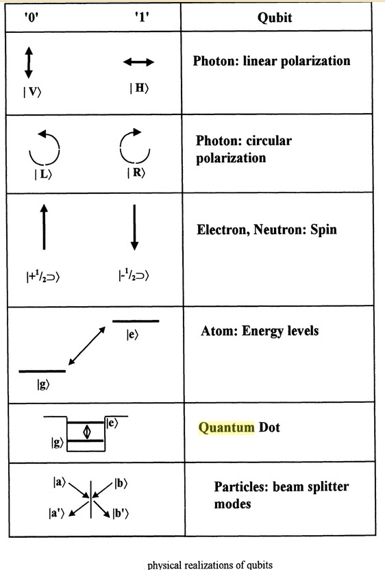
Qubits can be realised with multiple technologies, for example, quantum dots are structures that can confine and manipulate a single electron to be acted as a qubit. Another way of manipulating the spin of an electron is done via nitrogen-vacancy centers in diamond. Transmon qubits are one type of superconducting qubits that use Josephson junctions to create a single magnetic flux for use as a qubit. Ion-based qubits use ion traps to store qubits in individual ionised atoms suspended in a vacuum and controlled using lasers and electric and magnetic fields. Qubits can also be achieved by controlling the polarisation of photons, or the number of photons. Unlike classical computing, qubits can be in 1, 0 or in a superposition of 1 or 0 quantum states until we measure them. Following this logic, a pair of qubits can be in any quantum superposition of four states and three qubits will be in any superposition of 8 states. By extrapolation, we can generalise that n qubits will be in a superposition of up to 2^n different quantum states simultaneously. It is this simultaneity property that leads us to a potential quantum advantage. If we can use this massive parallelism, we can compute many operations at the same time, thus inferring a time advantage.

_

The superconducting qubit or transmon is already in use in some early-stage commercial quantum computer prototypes from IBM and Google. A transmon is a sort of artificial atom built from materials such as niobium and aluminum that, at low temperatures, can carry electrical current without resistance. These materials are patterned to form a small electrical circuit that behaves like an atom. The state of the qubit, the quantum 0 or 1, is represented by the amount of energy stored in the artificial atom.

Another strategy for making qubits involves real atoms. Jeffrey Thompson, assistant professor of electrical engineering, cools atoms down to incredibly low temperatures and traps them in a vacuum chamber. Once isolated, the researchers can manipulate an individual atom with tightly focused laser beams called optical tweezers. The researchers can then use additional laser signals to set the trapped atom’s energy levels to represent quantum 0 or 1 states. “Atoms make very good qubits,” Thompson said. “They are actually easy to work with, and it’s very easy to see a single atom using laser light.”

Still another type of qubit relies on electrons, or more specifically, an inherent quantum property of electrons known as spin. Spin describes the electron’s angular momentum and is sometimes likened to the twirling movement of a top, but it is also analogous to magnetism because, like a magnet, an electron’s spin can point either downward or upward, representing the values of 0 and 1.

Stephen Lyon, professor of electrical engineering, is one of the researchers exploring ways to keep spin qubits in superposition for relatively long periods. His team sends microwave pulses through a highly purified type of silicon, called silicon-28, to coordinate the spins of millions of electrons. The researchers have shown that they can keep spin qubits in superposition for up to 10 seconds, a lengthy duration in the quantum realm.

_

For quantum computing to achieve its full potential, qubits will not only need to keep their quantum states, but they will also need to share information with each other. They do this via a quantum property called entanglement. By entangling qubits, researchers can build quantum circuits that can do complex calculations. Jason Petta, the Eugene Higgins Professor of Physics, is working on this challenge for silicon-based spin qubits. Single spins can have a lifetime of up to one minute. Silicon spin qubits could prove less expensive and easier to manufacture than other types of qubits, and although they are not as far along in development as transmons, they are quickly catching up due to recent advances.

Petta’s team is devising ways to transfer the information coded in the electron’s spin from one qubit to another — getting electrons to, as he calls it, “talk to each other.” They build qubits by confining electrons in tiny silicon chambers called quantum dots. The researchers can then apply a strong magnetic field to the dots to coax them to transfer their quantum information to particles of light, or photons, which act as messengers to carry the information to other quantum dots located nearby. This strategy has already been used to entangle superconducting qubits, and the Petta group showed that this approach also works for spin-based qubits. “It’s like putting an electron and a photon in the same room,” Petta said. “You can transfer some of the spin properties to the photon, which is flying around the room, and then use the photon to transmit information to another spin on the opposite side of the room.”

The variety of ways of producing qubits underscores the state of quantum computing today. One of the more long-term strategies is to make qubits from Majorana fermions, which are particle-like objects that form under specific conditions. Predicted nearly a century ago, these quasi-particles were recently observed in experiments led by Ali Yazdani. The properties of these quasi-particles stem from a branch of mathematics called topology, which describes how objects can be bent or stretched without losing their inherent properties. This property could give these topological qubits better protection from decoherence.

___

Synopsis of physical realizations of qubits:

For physically implementing a quantum computer, many different candidates are being pursued, among them (distinguished by the physical system used to realize the qubits):

1. Superconducting quantum computing (qubit implemented by the state of small superconducting circuits (Josephson junctions))
2. Trapped ion quantum computer (qubit implemented by the internal state of trapped ions)
3. Optical lattices (qubit implemented by internal states of neutral atoms trapped in an optical lattice)
4. Quantum dot computer, spin-based (e.g. the Loss-DiVincenzo quantum computer) (qubit given by the spin states of trapped electrons)
5. Quantum dot computer, spatial-based (qubit given by electron position in double quantum dot)
6. Coupled Quantum Wire (qubit implemented by a pair of Quantum Wires coupled by a Quantum Point Contact)
7. Nuclear magnetic resonance quantum computer (NMRQC) implemented with the nuclear magnetic resonance of molecules in solution, where qubits are provided by nuclear spins within the dissolved molecule and probed with radio waves
8. Solid-state NMR Kane quantum computers (qubit realized by the nuclear spin state of phosphorus donors in silicon)
9. Electrons-on-helium quantum computers (qubit is the electron spin)
10. Cavity quantum electrodynamics (CQED) (qubit provided by the internal state of trapped atoms coupled to high-finesse cavities)
11. Molecular magnet (qubit given by spin states)
12. Fullerene-based ESR quantum computer (qubit based on the electronic spin of atoms or molecules encased in fullerenes)
13. Linear optical quantum computer (qubits realized by processing states of different modes of light through linear elements e.g. mirrors, beam splitters and phase shifters)
14. Diamond-based quantum computer (qubit realized by the electronic or nuclear spin of nitrogen-vacancy centers in diamond)
15. Bose-Einstein condensate-based quantum computer
16. Transistor-based quantum computer – string quantum computers with entrainment of positive holes using an electrostatic trap
17. Rare-earth-metal-ion-doped inorganic crystal based quantum computers (qubit realized by the internal electronic state of dopants in optical fibers)
18. Metallic-like carbon nanospheres based quantum computers

A large number of candidates demonstrates that the topic, in spite of rapid progress, is still in its infancy. There is also a vast amount of flexibility.

__

Figure below shows number of Qubits achieved by Date and Organization:

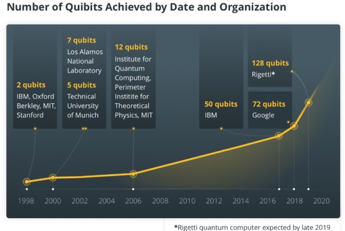
When trying to predict the future progress of quantum computers, the qubit count is often used as the primary indicator. This is misleading as there are other parameters that can inhibit the progress of quantum computers, even when the qubit count continues to increase. One of the biggest challenges is the need to perform 2-qubit operations on any 2 qubits, which is called qubit connectivity. Even in small quantum computer platforms that employ a single digit qubit count, such as the IBM Q experience, not all qubits are connected. This significantly reduces the ability to run complex quantum algorithms. Clearly, when scaling up the number of qubits, the qubit connectivity issue becomes even more challenging.

______

Two technologies are currently in the short-term lead:

1. Superconducting Qubits (IBM, Google, Rigetti, Alibaba, Intel, and Quantum Circuits). The basic element is a two-level energy system of a superconducting circuit which forms a somewhat noise-resistant qubit (a so-called transmon, first developed at Yale University—the alma mater of many key people in superconducting qubits R&D).

At every point of a superconducting electronic circuit (that is a network of electrical elements), the condensate wave function describing the charge flow is well-defined by a specific complex probability amplitude. In a normal conductor electrical circuit, the same quantum description is true for individual charge carriers, however the various wave functions are averaged in the macroscopic analysis, making it impossible to observe quantum effects. The condensate wave function allows designing and measuring macroscopic quantum effects. Superconducting circuits (so-called SQUIDs, or superconducting quantum interference devices) display macroscopically observable quantum properties.  For example, only a discrete number of magnetic flux quanta penetrates a superconducting loop, similarly to the discrete atomic energy levels in the Bohr model. In both cases, the quantization is a result of the complex amplitude continuity. Differing from the microscopic quantum systems (such as atoms or photons) used for implementations of quantum computers, the parameters of the superconducting circuits may be designed by setting the (classical) values of the electrical elements that compose them, e.g. adjusting the capacitance or inductance.

In order to obtain a quantum mechanical description of an electrical circuit a few steps are required. First, all the electrical elements are described with the condensate wave function amplitude and phase, rather than with the closely related macroscopic current and voltage description used for classical circuits. For example, a square of the wave function amplitude at some point in space is the probability of finding a charge carrier there, hence the square of the amplitude corresponds to the classical charge distribution. Second, generalized Kirchhoff’s circuit laws are applied at every node of the circuit network to obtain the equations of motion. Finally, the equations of motion are reformulated to Lagrangian mechanics and a quantum Hamiltonian is derived.

The devices are typically designed in the radio-frequency spectrum, cooled down in dilution refrigerators below 100mK and addressed with conventional electronic instruments, e.g. frequency synthesizers and spectrum analyzers. Typical dimensions on the scale of micrometers, with sub-micrometer resolution, allow a convenient design of a quantum Hamiltonian with the well-established integrated circuit technology.

A distinguishing feature of superconducting quantum circuits is the usage of a Josephson junction – an electrical element non existent in normal conductors. A junction is a weak connection between two leads of a superconducting wire, usually implemented as a thin layer of insulator with a shadow evaporation technique. The condensate wave functions on the two sides of the junction are weakly correlated – they are allowed to have different superconducting phases, contrary to the case of a continuous superconducting wire, where the superconducting wave function must be continuous. The current through the junction occurs by quantum tunneling. This is used to create a non-linear inductance which is essential for qubit design, as it allows a design of anharmonic oscillators. A quantum harmonic oscillator cannot be used as a qubit, as there is no way to address only two of its states.

2. Ion Traps (IonQ, Alpine Quantum Technologies, Honeywell, and others). The core elements are single ions (charged atoms) trapped in magnetic fields and the energy levels of their intrinsic spin form the qubit.

An ion trap quantum computer was first proposed by Cirac and Zoller in 1995 and implemented first by Monroe and collaborators in 1995 and then by Schwarzchild in 1996. The ion trap computer encodes data in energy states of ions and in vibrational modes between the ions. Conceptually each ion is operated by a separate laser. A preliminary analysis demonstrated that Fourier transforms can be evaluated with the ion trap computer. This, in turn, leads to Shor’s factoring algorithm, which is based on Fourier transforms.

_

Other technologies besides trapped ion and superconducting quantum computers:

Since many technical challenges remain in scaling either trapped ion or superconducting quantum computers, a number of research groups are continuing to explore other approaches for creating qubits and quantum computers. These technologies are much less developed, and are still focused on creating single qubit and two qubit gates.

Photons have a number of properties that make them an attractive technology for quantum computers: they are quantum particles that interact weakly with their environment and with each other. This natural isolation from the environment makes them an obvious approach to quantum communication. This base communication utility, combined with excellent single-qubit gates with high fidelity means that many early quantum experiments were done using photons. One key challenge with photonic quantum computers is how to create robust two-qubit gates. Researchers are currently working on two approaches for this issue. In linear optics quantum computing, an effective strong interaction is created by a combination of single-photon operations and measurements, which can be used to implement a probabilistic two-qubit gate, which heralds when it was successful. A second approach uses small structures in semiconductor crystals for photon interaction, and can also be considered a type of semiconductor quantum computer. These structures can be naturally occurring, called “optically active defects,” or man-made, which are often a structure called a “quantum dot.”

Work on building small-scale linear photon computers has been successful, and there are a number of groups trying to scale up the size of these machines. One key scaling issue for these machines is the “size” of a photonic qubit. Because the photons used in photonic quantum computing typically have wavelengths that are around a micron, and because the photons move at the speed of light and are typically routed along one dimension of the optical chip, increasing the number of photons, and hence the number of qubits, to extremely large numbers in a photonic device is even more challenging than it is in systems with qubits that can be localized in space. However, arrays with many thousands of qubits are expected to be possible.

Neutral atoms are another approach for qubits that is very similar to trapped ions, but instead of using ionized atoms and exploiting their charge to hold the qubits in place, neutral atoms and laser tweezers are used. Like trapped ion qubits, optical and microwave pulses are used for qubit manipulation, with lasers also being used to cool the atoms before computation. In 2018, systems with 50 atoms have been demonstrated with relatively compact spacing between the atoms. These systems have been used as analog quantum computers, where the interactions between qubits can be controlled by adjusting the spacing between the atoms. Building gate-based quantum computers using this technology requires creating high-quality two-qubit operations and isolating these operations from other neighboring qubits. As of mid-2018, entanglement error rates of 3 percent have been achieved in isolated two-qubit systems. Scaling up a gate-based neutral atom system requires addressing many of the same issues that arise when scaling a trapped ion computer, since the control and measurement layers are the same. Its unique feature compared to trapped ions is its potential for building multidimensional arrays.

Semiconductor qubits can be divided into two types depending on whether they use photons or electrical signals to control qubits and their interactions. Optically gated semiconductor qubits typically use optically active defects or quantum dots that induce strong effective couplings between photons, while electrically gated semiconductor qubits use voltages applied to lithographically defined metal gates to confine and manipulate the electrons that form the qubits. While less developed than other quantum technologies, this approach is more similar to that used for current classical electronics, potentially enabling the large investments that have enabled the tremendous scalability of classical electronics to facilitate the scaling of quantum information processors. Scaling optically gated qubits requires improved uniformity and requires accommodation of the need to individually address optically each qubit. Electrically gated qubits are potentially very dense, but material issues have limited the quality of even single-qubit gates until recently. While high density may enable a very large number of qubits to be integrated on the chip, it exacerbates the problem of building a control and measurement plane for these types of qubits: providing the needed wiring while avoiding interference and crosstalk between control signals will be extremely challenging. Quantum computers based on semiconductor technology are yet another possibility. Quantum dots are tiny semiconductor particles a few nanometers in size, having optical and electronic properties that differ from larger particles due to quantum mechanics. In a common approach a discrete number of free electrons (qubits) reside within extremely small regions, known as quantum dots, and in one of two spin states, interpreted as 0 and 1. Although prone to decoherence, such quantum computers build on well-established, solid-state techniques and offer the prospect of readily applying integrated circuit “scaling” technology. In addition, large ensembles of identical quantum dots could potentially be manufactured on a single silicon chip. The chip operates in an external magnetic field that controls electron spin states, while neighbouring electrons are weakly coupled (entangled) through quantum mechanical effects. An array of superimposed wire electrodes allows individual quantum dots to be addressed, algorithms executed, and results deduced. Such a system necessarily must be operated at temperatures near absolute zero to minimize environmental decoherence, but it has the potential to incorporate very large numbers of qubits.

Another approach to quantum computing uses topological qubits. In this computer qubits are encoded in a system of anyons. “Anyons” are quasiparticles in 2-dimensional media obeying parastatistics (neither Fermi Dirac nor Bose Einstein). But in a way anyons are still closer to fermions, because a fermion like repulsion exists between them. The respective movement of anyons is described by braid group. The idea behind the topological quantum computer is to make use of the braid group properties that describe the motion of anyons in order to carry out quantum computations. It is claimed that such a computer should be invulnerable to quantum errors of the topological stability of anyons. In this system, operations on the physical qubits have extremely high fidelities because the qubit operations are protected by topological symmetry implemented at the microscopic level: error correction is done by the qubit itself. This will reduce and possibly eliminate the overhead of performing explicit quantum error correction. While this would be an amazing advance, topological qubits are the least developed technology platform. In mid-2018, there are many nontrivial steps that need to be done to demonstrate the existence of a topological qubit, including experimentally observing the basic structure that underlies these qubits. Once these structures are built and controlled in the lab, the error resilience properties of this approach might enable it to scale faster than the other approaches.

_

Figure below shows types of qubits being used today:

____

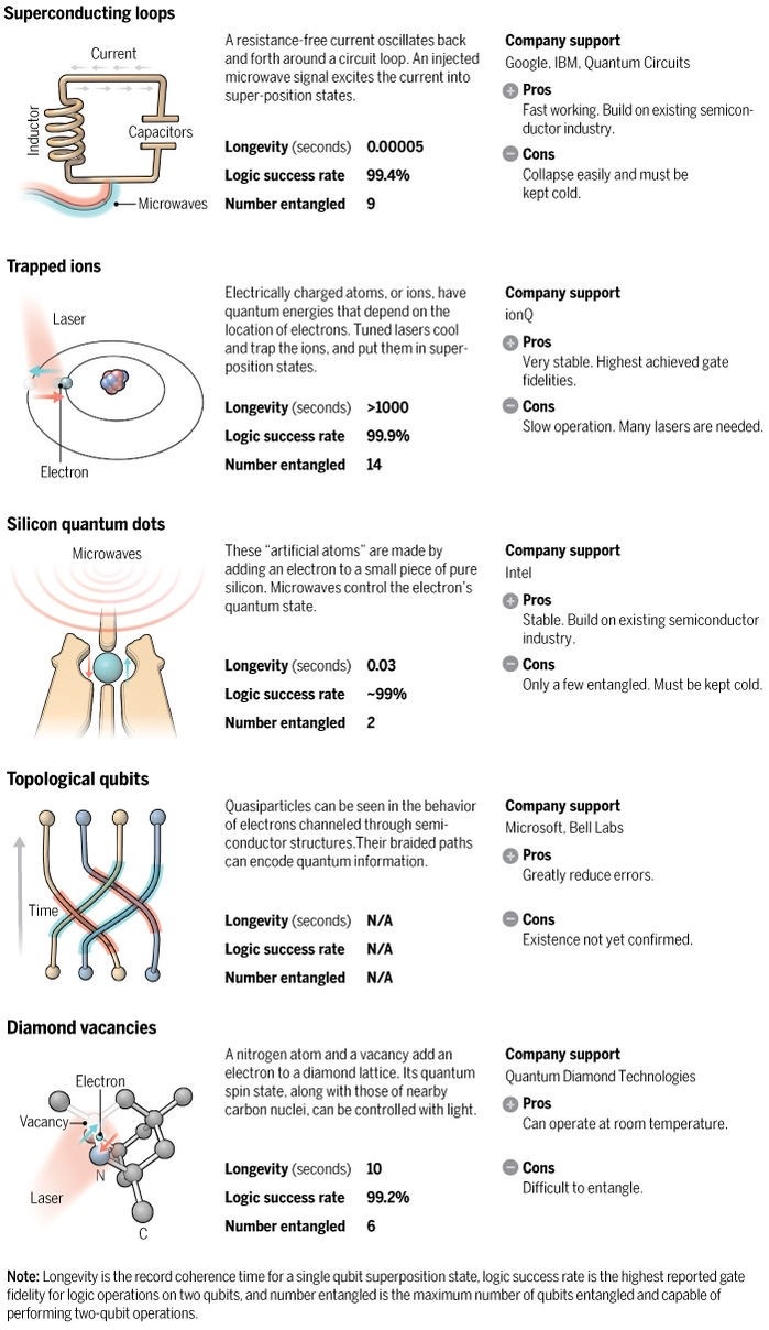
A silicon quantum computer:

The idea of using silicon-based CMOS technologies to build quantum computers was first proposed in 1998 by Bruce Kane, who was then a researcher at Australia’s University of New South Wales (UNSW). In his paper, Kane suggested that arrays of individual phosphorus atoms in crystalline silicon could store qubits in nuclear spins, and that these spin qubits could be read and manipulated using nuclear magnetic resonance techniques.

Noise is one of the great bugbears of quantum information processing, because it can make qubits change state at times and in ways that programmers did not intend, leading to computational errors. Most interactions with the surrounding environment, such as charge instabilities and thermal fluctuations, are sources of qubit noise. All of them can compromise information. Silicon, however, offers a relatively noise-free environment where spins can retain their quantum nature. The major source of unwanted quantum bit errors in silicon transistor-based qubits comes from the nuclear spins of silicon-29, a naturally occurring isotope present in all commercial silicon wafers. Luckily, purification methods can remove this unwanted isotope before the silicon crystals are grown, producing wafers of mostly spin-free silicon-28. For this reason, electron spins in silicon are among the most robust solid-state qubits available.

Following Kane’s seminal work, UNSW scientists continued to develop silicon-based quantum technology. They demonstrated (in 2012 and 2019, respectively) that single-qubit and two-qubit logic operations could indeed be carried out using phosphorous atoms. They also showed that qubits could be made by confining single spins in nanometer-size regions of the silicon chip known as quantum dots. The quantum dot approach is considered more practical than Kane’s original idea because it does not rely on atoms being positioned very precisely in an array. Instead, lithographic techniques are used to arrange the gate electrodes so that the QDs exist in a well-defined pattern.

____

Figure below shows different ways of building quantum computers:

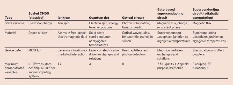
Source: A Blueprint for Building a Quantum Computer by Van Meter and Horsman.

_

To predict when we can expect a quantum computer to be operational we need to consider the hardware requirements of the specific quantum algorithm. These requirements can differ substantially depending on the type of calculation we want to perform. For example, to implement Shor’s algorithm for factoring a 2048 bit number we need more than 4000 stable qubits and billions of logical gates. As the duration of such a calculation will be much longer than the time that qubits can stay stable (coherence time), other techniques are then required to maintain the qubit information. These methods, such as quantum error correction, are far beyond the current capabilities of quantum computers. Therefore, even the most optimistic (without being unrealistic) predictions estimate a period of 10 years before the first demonstration of Shor’s algorithm on a 2048 bit number. On the other hand, the QAOA algorithm can outperform a classical computer with 100-200 qubit and a very shallow circuit depth (loosely defined as the number of logic gate operations), so quantum error correction is not strictly mandated. This is also the reason the QAOA is one of the candidates to demonstrate quantum supremacy.

_____

_____

General structure of a quantum computer system:

The quantum effect frequently, although not always, requires components operating near absolute zero, making just about every aspect of the design exotic. Quantum computer components operated at room temperature inevitably acquire error from the thermal motion of the atoms in the computers structure. The errors must be removed by quantum error correction, yet the error accumulation rate is too high for practical removal unless the components are cooled to millikelvins, or thousandths of a degree above absolute zero-273.15 °C or 0 K. The architecture of these quantum—classical hybrid computers is zeroing in on the structure shown in the figure below. The qubits (quantum bits) must be kept at a temperature of approximately 15 mK. They need support from classical superconducting electronics based on Josephson junctions operating at temperatures around helium’s boiling point, or 4K. The electronics must have extremely low energy dissipation, because the external refrigeration must dissipate at least the temperature ratio (300 K/4 K = 75x or 300 K/15 mK = 20,000x) times as much energy to remove the heat to room temperature (300 K)—and, in practice, several times this amount. Logic-gate circuits based on Josephson junctions are available that perform the logic functions for error correction as well as the gate microwave signals required to control qubits.

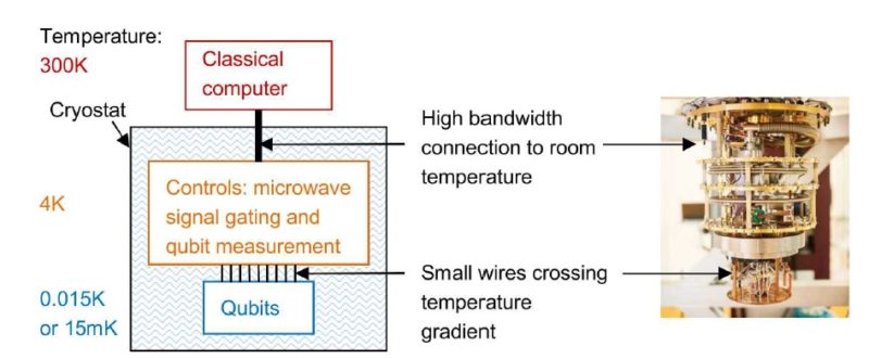
Figure above shows general structure of a quantum computer system. The user interacts with a classical computer. If the problem requires optimization, the classical computer translates the user’s problem into a standard form for a quantum computer, such as QUBO (Quadratic unconstrained binary optimization), or into a different form if another quantum algorithm is required. The classical computer then creates control signals for qubits (quantum bits) located in a cryogenic environment, receiving data from measurements of the qubits. Some classical electronics are placed in the cold environment to minimize heat flow through wiring across the cryogenic-to-room-temperature gradient.

_

Inside a quantum computer:

There are a few different ways to create a qubit. One method uses superconductivity to create and maintain a quantum state. To work with these superconducting qubits for extended periods of time, they must be kept very cold. Any heat in the system can introduce error, which is why quantum computers operate at temperatures close to absolute zero, colder than the vacuum of space.

Take a look at how a quantum computer’s dilution refrigerator, made from more than 2,000 components, creates such a cold environment for the qubits inside.

Here’s a look at how a quantum computer’s dilution refrigerator, made from more than 2,000 components, exploits the mixing properties of two helium isotopes to create such an environment for the qubits inside.

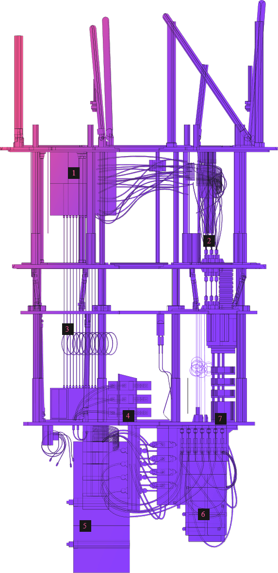
1. Qubit Signal Amplifier

One of two amplifying stages is cooled to a temperature of 4 Kelvin.

2. Input Microwave Lines

Attenuation is applied at each stage in the refrigerator in order to protect qubits from thermal noise during the process of sending control and readout signals to the processor.

3. Superconducting Coaxial Lines

In order to minimize energy loss, the coaxial lines that direct signals between the first and second amplifying stages are made out of superconductors.

4. Cryogenic Isolators

Cryogenic isolators enable qubits signals to go forward while preventing noise from compromising qubit quality.

5. Quantum Amplifiers

Quantum amplifiers inside of a magnetic shield capture and amplify processor readout signals while minimizing noise.

6. Cryoperm Shield

The quantum processor sits inside a shield that protects it from electromagnetic radiation in order to preserve its quality.

7. Mixing Chamber

The mixing chamber at the lowest part of the refrigerator provides the necessary cooling power to bring the processor and associated components down to a temperature of 15 mK — colder than outer space.

_

The inside of a quantum computer looks like a fancy gold chandelier. And, yes, it is made with real gold. It’s a dilution refrigerator that’s used to cool the quantum chips so that the computer can create superpositions and entangle qubits without losing any of the information as seen in the figure below.

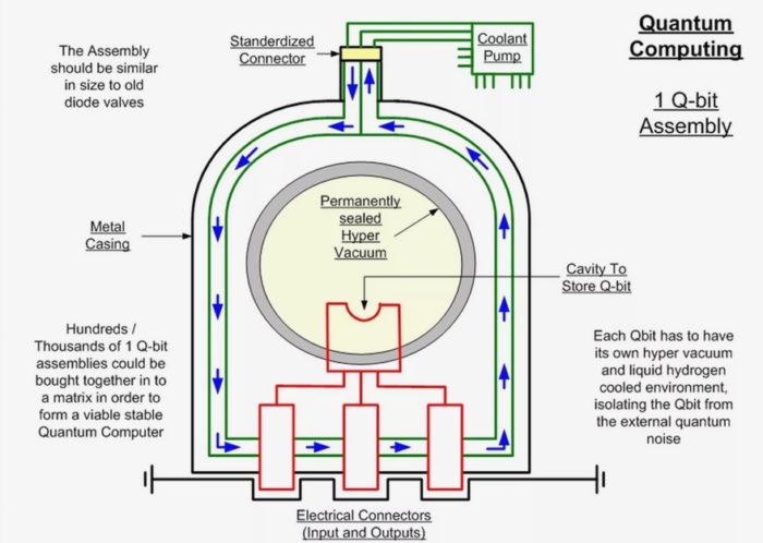
The quantum computer makes these qubits from any material that displays quantum mechanical properties that can be controlled. Quantum computing projects create qubits in different ways such as looping superconducting wire, spinning electrons, and trapping ions or pulses of photons. These qubits only exist in the sub-freezing temperatures created in the dilution refrigerator.

In practice, there are lots of possible ways of containing atoms/ions (qubits) and changing their states using laser beams, electromagnetic fields, radio waves, and an assortment of other techniques.

_____

Getting to know your quantum processor:

Quantum computers are built out of qubits. But just having lots of qubits is not enough. A billion qubits working in complete isolation will never achieve anything. They need to talk to each other. This means that the need to be connected by so-called controlled operations. Every device has its own rules for which pairs of qubits can be connected in this way. The better the connectivity of a device, the faster and easier it will be for us to implement powerful quantum algorithms. The nature of errors is also an important factor. In the near-term era of quantum computing, nothing will be quite perfect. So we need to know what kinds of errors will happen, how likely they are, and whether it is possible to mitigate their effects in the applications we care about. These are the three most important aspects of a quantum device: qubit number, connectivity and noise level. To have any idea of what a quantum computer can do, you need to know them all.

______

Horse Ridge chip from Intel:

Intel Labs in December 2019 unveiled what is believed to be a first of-its-kind cryogenic control chip — code-named Horse Ridge — that will speed up development of full stack quantum computing systems. The Horse Ridge chip addresses fundamental challenges in building a quantum system powerful enough to demonstrate quantum practicality: scalability, flexibility and fidelity.

Scalability: The integrated SoC design, implemented using Intel’s 22-nanometer FinFET Low Power CMOS technology, integrates four radiofrequency (RF) channels into a single device. Each channel is able to control up to 32 qubits by leveraging “frequency multiplexing” — a technique that divides the total bandwidth available into a series of non-overlapping frequency bands, each of which is used to carry a separate signal. With these four channels, Horse Ridge can potentially control up to 128 qubits with a single device, substantially reducing the number of cables and rack instrumentation previously required.

Fidelity: Increases in qubit count trigger other issues that challenge the capacity and operation of the quantum system. One such potential impact is a decline in qubit fidelity and performance. In developing Horse Ridge, Intel optimized the multiplexing technology that enables the system to scale and reduce errors from “phase shift” — a phenomenon that can occur when controlling many qubits at different frequencies, resulting in crosstalk among qubits. The engineers can tune various frequencies leveraged with Horse Ridge with high levels of precision, enabling the quantum system to adapt and automatically correct for phase-shift when controlling multiple qubits with the same RF line, improving qubit gate fidelity.

Flexibility: Horse Ridge can cover a wide frequency range, enabling control of both superconducting qubits (known as transmons) and spin qubits. Transmons typically operate around 6-7GHz, while spin qubits operate around 13-20GHz.

Intel’s ‘Horse Ridge’ greatly simplifies today’s complex control electronics required to operate such a quantum system by using a highly integrated system-on-chip (SoC) for faster set-up time, improved qubit performance and efficient scaling to larger qubit counts required for quantum computing to solve practical, real-world applications. The integrated SoC design integrates four radio frequency (RF) channels into a single device. Each channel is able to control up to 32 qubits, leveraging “frequency multiplexing”. Leveraging these four channels, Horse Ridge can potentially control up to 128 qubits with a single device, substantially reducing the number of cables and rack instrumentations previously required. Increases in qubit count trigger other issues like decline in qubit fidelity and performance. In developing ‘Horse Ridge’, Intel has optimised the multiplexing technology that enables the system to scale and reduce errors. Horse Ridge can cover a wide frequency range, enabling control of both superconducting qubits (known as transmons) and spin qubits.

Key Benefits:

1. Reduced form factor (chip and PCB size) and power required to operate quantum systems.
2. Ability to scale to and control a larger number of qubits (up to 128 qubits)
3. High flexibility in control pulses that can be generated with Horse Ridge reduces crosstalk among qubits with improved overall gate fidelity.
4. The device can automatically correct phase shift, which occurs when controlling multiple qubits at different frequencies with the same RF line, with a digital codeword update after each pulse of the control electronics.

_____

_____

Quantum software:

Qiskit Aqua — A Library of Quantum Algorithms and Applications:

Sitting atop the Qiskit ecosystem, Aqua is the element that encompasses cross-domain quantum algorithms and applications running on Noisy Intermediate-Scale Quantum (NISQ) computers. Aqua is an open-source library completely written in Python and specifically designed to be modular and extensible at multiple levels. As shown in figure below, this flexibility allows users with differing levels of experience and scientific interests to contribute to, and extend, Aqua throughout the stack.

_

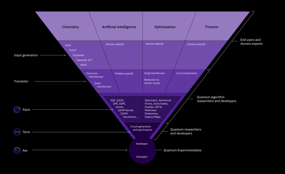
Figure above shows Aqua Software Stack:

With the addition of Aqua, Qiskit has become the only scientific software framework for quantum computing that is capable of taking high-level domain-specific problem specifications down to circuit generation, compilation, and finally execution on IBM Q quantum hardware.

Input Generation:

Currently, Aqua supports four applications, in domains that have long been identified as potential areas for quantum computing: Chemistry, Artificial Intelligence (AI), Optimization, and Finance. New domains can be easily added using the versatile Aqua interfaces. At this application level, Aqua allows for classical computational software to be leveraged as the quantum application front-end, without the need for the end user to learn a new programming language. Behind the scenes, Aqua employs hybrid classical/quantum processes; some initial computation is performed classically, and the results of those computations are then combined with problem-specific configuration data, and translated into inputs for one or more quantum algorithms. The Aqua algorithms run on top of Terra, the element of Qiskit responsible for building, compiling and executing quantum circuits on simulators or real quantum devices.

Quantum Algorithms on Aqua:

Researchers focusing on quantum algorithms can experiment with many algorithms made readily available in Aqua. These include numerous domain-independent algorithms, such as the VQE algorithm, the Quantum Approximate Optimization Algorithm (QAOA), Grover’s Search Algorithm, and various forms of Quantum Phase Estimation (QPE). In addition, domain-specific algorithms, such as the Support Vector Machine (SVM) Quantum Kernel and Variational algorithms, suitable for supervised learning, are also available. It is also possible for researchers to contribute their own algorithms by extending the Aqua Quantum Algorithm interface. These efforts are aided by a vast set of supporting components, such as local and global optimizers, variational forms, initial states for variational-form initialization, Inverse Quantum Fourier Transforms (IQFTs), oracles, feature maps, and binary-to-multiclass classification extensions. To facilitate the integration of new components, Aqua includes an automatic component-discovery mechanism that allows components to register themselves for dynamical loading at run time.

User Experience:

Utilizing classical computational software at the front end of Aqua has unique advantages. Users at the top of the Aqua software stack are industry-domain experts, who are most likely very familiar with existing classical software specific to their own domains, such as the PySCF computational chemistry software driver used in the code. These practitioners are interested in experimenting with the potential benefits of quantum computing, but at the same time they might be hesitant to learn the intricate details of the underlying quantum physics. Ideally, such practitioners would benefit from a workflow centered around the computational software they are comfortable with as the front end, without having to learn a new quantum programming language or Application Programming Interface (API). Moreover, such researchers may have collected, over time, numerous problem configurations, corresponding to various experiments that are all tied to a specific classical computational package. Aqua has been designed from the outset to accept input files in the language of any classical computational package it interfaces, thus not requiring users experienced in a particular domain to learn a new quantum-specific language for the same task.

Functionality:

While other quantum software libraries impose an intermediate programming layer or API between the classical and quantum parts of a hybrid program, Aqua is unique in its ability to directly interface with classical computational software, thus allowing for the computation of the intermediate data needed to construct the quantum-algorithm input to be performed at its highest level of precision, all without losing any functionality inherent in the underlying classical software.

______

Besides qubits, and in order to operate a quantum computer, we need the full quantum hardware and software layer stack as seen in the figure below.

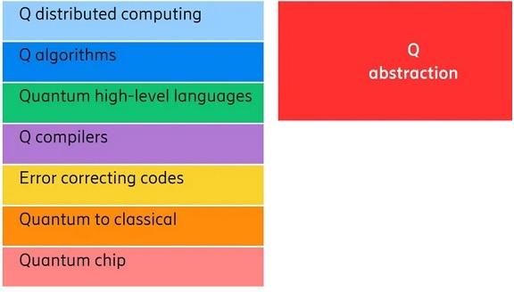
Figure above shows Quantum computer hardware and software stack.

______

Current state of quantum computing:

We are in the era of NISQ — Noisy Intermediate Scale Quantum devices. This means, that even though we are talking about 20–70 qubits, they are so crappy, that you can’t do anything useful with them. The first reason for that is that they are extremely sensitive to all types of noise — that’s one of the reasons why they need to operate in the temperature of 15 mK. And every interaction with the outside world might end up with the destruction of the quantum state. The second reason is that you usually can’t make two arbitrary qubits interact with each other — and this limits their computational power significantly. The third reason is that in order to be useful, these machines have to outcompete regular computers which have at least a 50 years head start. And keep in mind, that the “crappy” machines we are talking about here are marvels of contemporary engineering, with dedicated teams of people working on refining this technology.

______

______

Challenges for Quantum Computing:

Quantum computing is a new and promising technology with the potential of exponentially powerful computation – if only a large-scale one can be built. There are several challenges in building a large-scale quantum computer – fabrication, verification, and architecture. The power of quantum computing comes from the ability to store a complex state in a single bit. This also what makes quantum systems difficult to build, verify, and design. Quantum states are fragile, so fabrication must be precise, and bits must often operate at very low temperatures. Unfortunately, the complete state may not be measured precisely, so verification is difficult. Imagine verifying an operation that is expected to not always get the same answer, but only an answer with a particular probability! Finally, errors occur much more often than with classical computing, making error correction the dominant task that quantum architectures need to perform well.

_

Quantum computers are extremely temperamental machines, which makes them immensely difficult to build and operate. They need to be isolated from the outside environment and kept almost at absolute zero (-273ºC) in order to be usable. If not, they produce quantum decoherence, which is essentially the loss of information to the environment. Quantum decoherence can even be generated within the system itself, through the effects of things like background thermonuclear spin or lattice vibration. Once quantum decoherence is introduced to a system, it cannot be removed, which is why quantum computers need to be so tightly controlled in order to be usable. At this stage, numerous technological challenges need to be surpassed in order to produce a sizable quantum computer with minimal quantum decoherence.

_

Most quantum computers require temperatures colder than those found in deep space. To reach these temperatures, all the components and hardware are contained within a dilution refrigerator—highly specialized equipment that cools the qubits to just above absolute zero. Because standard electronics don’t work at these temperatures, a majority of quantum computers today use room-temperature control. With this method, controls on the outside of the refrigerator send signals through cables, communicating with the qubits inside. The challenge is that this method ultimately reaches a roadblock: the heat created by the sheer number of cables limits the output of signals, restraining the number of qubits that can be added.

As more control electronics are added, more effort is needed to maintain the very low temperature the system requires. Increasing both the size of the refrigerator and the cooling capacity is a potential option, however, this would require additional logistics to interface with the room temperature electronics, which may not be a feasible approach.

Another alternative would be to break the system into separate refrigerators. Unfortunately, this isn’t ideal either because the transfer of quantum data between the refrigerators is likely to be slow and inefficient.

At this stage in the development of quantum computers, size is therefore limited by the cooling capacity of the specialized refrigerator. Given these parameters, the electronics controlling the qubits must be as efficient as possible.

_

A quantum computer holds the promise to solve efficiently some classes of computational problems that are intractable for a classical computer by using quantum algorithms that exploit fundamental quantum phenomena such are superposition and entanglement. The most famous example is the factorisation of large numbers using Shor’s algorithm, which is exponentially faster than its best classical counterpart. By running this algorithm on a quantum computer we could factorize, for instance a 2000-bit number but such a quantum computer would require around millions or even billions of physical quantum bits or qubits. That large number of qubits mainly comes from the need to deal with the fragility of the quantum technology and to make quantum systems robust against errors. Qubits suffer from decoherence meaning that the information stored in the qubits is lost due to the interaction with the environment, leading to gate error rates of around ∼ 10−². However, quantum systems can be protected and recovered from such errors by using quantum error correction (QEC) and fault tolerant (FT) computations if the gate error rates are below a certain threshold. These procedures will be essential for any quantum computer but they will also dramatically increase the amount of qubits required for computation. Building a full scale quantum computer is therefore directly influenced by the above observations and basically fall apart in two challenges: to increase the fidelity of quantum operations and to scale the control infrastructure of large numbers of qubits in the range of millions.

_

To put the hardware challenges in perspective, we need:

1. Moderately more qubits. 64, 128, 192, 256, 512, 1024. As a start.
2. Much larger numbers of qubits — tens of thousands, hundreds of thousands, even millions. A 1,000 by 1,000 lattice (grid) is one million qubits, but is still a rather modest amount of data by today’s standards.
3. Much greater connectivity (entanglement) with far fewer, if any, restrictions.
4. Much lower error rate.
5. Much longer coherence.
6. Much greater circuit depth.
7. True fault tolerance — error correction, which requires significant redundancy for each qubit.
8. Much lower cost for the full system.
9. Non-cryogenic operating temperatures.
10. Easy sourcing for quantum computers parts: Quantum computers need Helium-3, a nuclear research by-product, and special cables that are only made by a single company in Japan.

Granted, selective niche problems can achieve adequate solutions without a good fraction of those needed advances, but true, general-purpose, widely-usable, practical quantum computers will require most of those advances.

____

There are few key challenges that could keep quantum computing from becoming a reality. But if solved, we could create a commercially relevant quantum computer in about 10-12 years, a computer that might change our lives.

1. Qubit Quality: We need to make qubits that we will be able to generate useful instructions or gate operations for on a large scale and we are not there yet. Even the few qubits in today’s cloud-based quantum computers are not good enough for large scale systems. They still generate errors when running operations between two qubits at a rate that is far higher than what we would need to effectively compute. In other words, after a certain number of instructions or operations, today’s qubits produce the wrong answer when we run calculations. The result we get can be indistinguishable from noise.
2. Error Correction: Now, because qubits aren’t quite good enough for the scale we need them to operate at, we need to implement error correction algorithms that check and then correct for random qubit errors as they occur. These are complex instruction sets that use many physical qubits to effectively extend the lifetime of the information in the system.
3. Qubit Control: In order to implement complex algorithms, including error correction schemes, we need to prove that we can control multiple qubits. That control must have low-latency—on the order of 10’s of nanoseconds. And it must come from CMOS-based adaptive feedback control circuits.
4. Too Many Wires: Today, we require multiple control wires, or multiple lasers, to create each qubit. It is difficult to believe that we could build a million-qubit chip with many millions of wires connecting to the circuit board or coming out of the cryogenic measurement chamber. In fact, the semiconductor industry recognized this problem in the mid-1960s and designated it Rent’s Rule. Put another way, we will never drive on the quantum highway without well designed roads.
5. Decoherence: Sensitivity to interaction with the environment: Quantum computers are extremely sensitive to interaction with the surroundings since any interaction (or measurement) leads to a collapse of the state function. This phenomenon is called decoherence. It is extremely difficult to isolate a quantum system, especially an engineered one for a computation, without it getting entangled with the environment. The larger the number of qubits the harder is it to maintain the coherence.

Quantum decoherence is the loss of quantum coherence. In quantum mechanics, particles such as electrons are described by a wave function, a mathematical representation of the quantum state of a system; a probabilistic interpretation of the wave function is used to explain various quantum effects. As long as there exists a definite phase relation between different states, the system is said to be coherent. A definite phase relationship is necessary to perform quantum computing on quantum information encoded in quantum states. Coherence is preserved under the laws of quantum physics.

One of the greatest challenges is controlling or removing quantum decoherence. This usually means isolating the system from its environment as interactions with the external world cause the system to decohere. However, other sources of decoherence also exist. Examples include the quantum gates, and the lattice vibrations and background thermonuclear spin of the physical system used to implement the qubits. Decoherence is irreversible, as it is effectively non-unitary, and is usually something that should be highly controlled, if not avoided. Decoherence times for candidate systems in particular, the transverse relaxation time T₂ (for NMR and MRI technology, also called the dephasing time), typically range between nanoseconds and seconds at low temperature. Currently, some quantum computers require their qubits to be cooled to 20 millikelvins in order to prevent significant decoherence.  As a result, time-consuming tasks may render some quantum algorithms inoperable, as maintaining the state of qubits for a long enough duration will eventually corrupt the superpositions.  These issues are more difficult for optical approaches as the timescales are orders of magnitude shorter and an often-cited approach to overcoming them is optical pulse shaping. Error rates are typically proportional to the ratio of operating time to decoherence time, hence any operation must be completed much more quickly than the decoherence time.

6. Unreliable quantum gate actions: Quantum computation on qubits is accomplished by operating upon them with an array of transformations that are implemented in principle using small gates. It is imperative that no phase errors be introduced in these transformations. But practical schemes are likely to introduce such errors. It is also possible that the quantum register is already entangled with the environment even before the beginning of the computation. Furthermore, uncertainty in initial phase makes calibration by rotation operation inadequate. In addition, one must consider the relative lack of precision in the classical control that implements the matrix transformations. This lack of precision cannot be completely compensated for by the quantum algorithm.
7. Constraints on state preparation: State preparation is the essential first step to be considered before the beginning of any quantum computation. In most schemes, the qubits need to be in a particular superposition state for the quantum computation to proceed correctly. But creating arbitrary states precisely can be exponentially hard (in both time and resource (gate) complexity).
8. Quantum information, uncertainty, and entropy of quantum gates: Classical information is easy to obtain by means of interaction with the system. On the other hand, the impossibility of cloning means that any specific unknown state cannot be determined. This means that unless the system has specifically been prepared, our ability to control it remains limited. The average information of a system is given by its entropy. The determination of entropy would depend on the statistics obeyed by the object.

______

Noise and error correction:

The mathematics that underpin quantum algorithms is well established, but there are daunting engineering challenges that remain. For computers to function properly, they must correct all small random errors. In a quantum computer, such errors arise from the non-ideal circuit elements and the interaction of the qubits with the environment around them. For these reasons the qubits can lose coherency in a fraction of a second and, therefore, the computation must be completed in even less time. If random errors – which are inevitable in any physical system – are not corrected, the computer’s results will be worthless.

In classical computers, small noise is corrected by taking advantage of a concept known as thresholding. It works like the rounding of numbers. Thus, in the transmission of integers where it is known that the error is less than 0.5, if what is received is 3.45, the received value can be corrected to 3. Further errors can be corrected by introducing redundancy. Thus if 0 and 1 are transmitted as 000 and 111, then at most one bit-error during transmission can be corrected easily: A received 001 would be a interpreted as 0, and a received 101 would be interpreted as 1.

Quantum error correction codes are a generalization of the classical ones, but there are crucial differences. For one, the unknown qubits cannot be copied to incorporate redundancy as an error correction technique. Furthermore, errors present within the incoming data before the error-correction coding is introduced cannot be corrected.

_

Graphic of Quantum Errors:

_

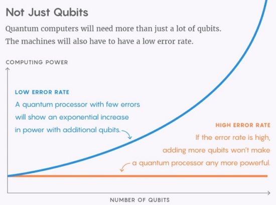
Physical qubits, logical qubits, and the role of error correction:

By nature, qubits are fragile. They require a precise environment and state to operate correctly, and they’re highly prone to outside interference. This interference is referred to as ‘noise’, which is a consistent challenge and a well-known reality of quantum computing. As a result, error correction plays a significant role.

As a computation begins, the initial set of qubits in the quantum computer are referred to as physical qubits. Error correction works by grouping many of these fragile physical qubits, which creates a smaller number of usable qubits that can remain immune to noise long enough to complete the computation. These stronger, more stable qubits used in the computation are referred to as logical qubits.

A lot of research on the fundamentals of quantum computing has been devoted to error correction. Part of the difficulty stems from another of the key properties of quantum systems: Superpositions can only be sustained as long as you don’t measure the qubit’s value. If you make a measurement, the superposition collapses to a definite value: 1 or 0. So how can you find out if a qubit has an error if you don’t know what state it is in? One ingenious scheme involves looking indirectly, by coupling the qubit to another “ancilla” qubit that doesn’t take part in the calculation but that can be probed without collapsing the state of the main qubit itself. It’s complicated to implement, though. Such solutions mean that, to construct a genuine “logical qubit” on which computation with error correction can be performed, you need many physical qubits.

How many? Quantum theorist Alán Aspuru-Guzik of Harvard University estimates that around 10,000 of today’s physical qubits would be needed to make a single logical qubit — a totally impractical number. If the qubits get much better, he said, this number could come down to a few thousand or even hundreds. Eisert is less pessimistic, saying that on the order of 800 physical qubits might already be enough, but even so he agrees that “the overhead is heavy,” and for the moment we need to find ways of coping with error-prone qubits.

In classical computing, noisy bits are fixed through duplication (parity and Hamming codes), which is a way to correct errors as they occur. A similar process occurs in quantum computing, but is more difficult to achieve. This results in significantly more physical qubits than the number of logical qubits required for the computation. The ratio of physical to logical qubits is influenced by two factors: 1) the type of qubits used in the quantum computer, and 2) the overall size of the quantum computation performed. And due to the known difficulty of scaling the system size, reducing the ratio of physical to logical qubits is critical. This means that instead of just aiming for more qubits, it is crucial to aim for better qubits.

Stability and scale with a topological qubit:

The topological qubit is a type of qubit that offers more immunity to noise than many traditional types of qubits. Topological qubits are more robust against outside interference, meaning fewer total physical qubits are needed when compared to other quantum systems. With this improved performance, the ratio of physical to logical qubits is reduced, which in turn, creates the ability to scale. If topological qubits were used in the example of nitrogenase simulation, the required 200 logical qubits would be built out of thousands of physical qubits. However, if more traditional types of qubits were used, tens or even hundreds of thousands of physical qubits would be needed to achieve 200 logical qubits. The topological qubit’s improved performance causes this dramatic difference; fewer physical qubits are needed to achieve the logical qubits required. Developing a topological qubit is extremely challenging and is still underway, but these benefits make the pursuit well worth the effort.

_

Quantum threshold theorem:

In quantum computing, the (quantum) threshold theorem (or quantum fault-tolerance theorem), proved by Michael Ben-Or and Dorit Aharonov states that a quantum computer with a physical error rate below a certain threshold can, through application of quantum error correction schemes, suppress the logical error rate to arbitrarily low levels. Current estimates put the threshold for the surface code on the order of 1%, though estimates range widely and are difficult to calculate due to the exponential difficulty of simulating large quantum systems.  Error rates are typically proportional to the ratio of operating time to decoherence time, hence any operation must be completed much more quickly than the decoherence time.  As described in the Quantum threshold theorem, if the error rate is small enough, it is thought to be possible to use quantum error correction to suppress errors and decoherence. This allows the total calculation time to be longer than the decoherence time if the error correction scheme can correct errors faster than decoherence introduces them. An often cited figure for the required error rate in each gate for fault-tolerant computation is 10⁻³, assuming the noise is depolarizing. At a 0.1% probability of a depolarizing error, the surface code would require approximately 1,000-10,000 physical qubits per logical data qubit, though more pathological error types could change this figure drastically.

According to leading quantum information theorist Scott Aaronson:

“The entire content of the Threshold Theorem is that you’re correcting errors faster than they’re created. That’s the whole point, and the whole non-trivial thing that the theorem shows. That’s the problem it solves.”

_

Quantum error correction:

Quantum error correction (QEC) is used in quantum computing to protect quantum information from errors due to decoherence and other quantum noise. Quantum error correction is essential if one is to achieve fault-tolerant quantum computation that can deal not only with noise on stored quantum information, but also with faulty quantum gates, faulty quantum preparation, and faulty measurements.

Classical error correction employs redundancy. The simplest way is to store the information multiple times, and—if these copies are later found to disagree—just take a majority vote; e.g. suppose we copy a bit three times. Suppose further that a noisy error corrupts the three-bit state so that one bit is equal to zero but the other two are equal to one. If we assume that noisy errors are independent and occur with some probability p, it is most likely that the error is a single-bit error and the transmitted message is three ones. It is possible that a double-bit error occurs and the transmitted message is equal to three zeros, but this outcome is less likely than the above outcome.

Copying quantum information is not possible due to the no-cloning theorem. This theorem seems to present an obstacle to formulating a theory of quantum error correction. But it is possible to spread the information of one qubit onto a highly entangled state of several (physical) qubits. Peter Shor first discovered this method of formulating a quantum error correcting code by storing the information of one qubit onto a highly entangled state of nine qubits. A quantum error correcting code protects quantum information against errors of a limited form.

Classical error correcting codes use a syndrome measurement to diagnose which error corrupts an encoded state. We then reverse an error by applying a corrective operation based on the syndrome. Quantum error correction also employs syndrome measurements. We perform a multi-qubit measurement that does not disturb the quantum information in the encoded state but retrieves information about the error. A syndrome measurement can determine whether a qubit has been corrupted, and if so, which one. What is more, the outcome of this operation (the syndrome) tells us not only which physical qubit was affected, but also, in which of several possible ways it was affected. The latter is counter-intuitive at first sight: Since noise is arbitrary, how can the effect of noise be one of only few distinct possibilities? In most codes, the effect is either a bit flip, or a sign (of the phase) flip, or both (corresponding to the Pauli matrices X, Z, and Y). The reason is that the measurement of the syndrome has the projective effect of a quantum measurement. So even if the error due to the noise was arbitrary, it can be expressed as a superposition of basis operations—the error basis (which is here given by the Pauli matrices and the identity). The syndrome measurement “forces” the qubit to “decide” for a certain specific “Pauli error” to “have happened”, and the syndrome tells us which, so that we can let the same Pauli operator act again on the corrupted qubit to revert the effect of the error.

The syndrome measurement tells us as much as possible about the error that has happened, but nothing at all about the value that is stored in the logical qubit—as otherwise the measurement would destroy any quantum superposition of this logical qubit with other qubits in the quantum computer.

Because truly isolating a quantum system has proven so difficult, error correction systems for quantum computations have been developed. Qubits are not digital bits of data, thus they cannot use conventional (and very effective) error correction, such as the triple redundant method. Given the nature of quantum computing, error correction is ultra critical – even a single error in a calculation can cause the validity of the entire computation to collapse. There has been considerable progress in this area, with an error correction algorithm developed that utilizes 9 qubits (1 computational and 8 correctional). More recently, there was a breakthrough by IBM that makes do with a total of 5 qubits (1 computational and 4 correctional).

__

What is a classical bit? The electricity flows or doesn’t flow. Even if the current weakens or becomes stronger, it is still considered a current. The quantum bits are sequential, the electron can be largely in atom right and partially in atom left. That is their strength and that is their weakness. Therefore, every interaction with the environment affects them dramatically. If you use your regular computer and an electronic wave passes through the transistor, the state of the bit does not change. The same electronic wave passing through a qubit will cause loss of the qubit’s coherence, memory. The information will leak out to the surroundings and we will not be able to reconstruct it.

A classical processor performs a calculation in a nanosecond, but will preserve the information for days, months, years ahead. A quantum computer also performs a calculation in a nanosecond – and at best will manage to preserve the information for a hundredth of a microsecond. Quantum computers are so sensitive to external interference that they must be isolated from their surroundings at almost minus 273 degrees Celsius, one 10,000th of a degree above absolute zero.

One way of correcting errors is avoiding them or cancelling out their influence: so-called error mitigation. Researchers at IBM, for example, are developing schemes for figuring out mathematically how much error is likely to have been incurred in a computation and then extrapolating the output of a computation to the “zero noise” limit.

Some researchers think that the problem of error correction will prove intractable and will prevent quantum computers from achieving the grand goals predicted for them. “The task of creating quantum error-correcting codes is harder than the task of demonstrating quantum supremacy,” said mathematician Gil Kalai of the Hebrew University of Jerusalem in Israel. And he adds that “devices without error correction are computationally very primitive, and primitive-based supremacy is not possible.” In other words, you’ll never do better than classical computers while you’ve still got errors.

Others believe the problem will be cracked eventually. According to Jay Gambetta, a quantum information scientist at IBM’s Thomas J. Watson Research Center, “Our recent experiments at IBM have demonstrated the basic elements of quantum error correction on small devices, paving the way towards larger-scale devices where qubits can reliably store quantum information for a long period of time in the presence of noise.” Even so, he admits that “a universal fault-tolerant quantum computer, which has to use logical qubits, is still a long way off.” Such developments make Childs cautiously optimistic. “I’m sure we’ll see improved experimental demonstrations of [error correction], but I think it will be quite a while before we see it used for a real computation,” he said.

Living with Errors:

For the time being, quantum computers are going to be error-prone, and the question is how to live with that. At IBM, researchers are talking about “approximate quantum computing” as the way the field will look in the near term: finding ways of accommodating the noise.

This calls for algorithms that tolerate errors, getting the correct result despite them. It’s a bit like working out the outcome of an election regardless of a few wrongly counted ballot papers. “A sufficiently large and high-fidelity quantum computation should have some advantage [over a classical computation] even if it is not fully fault-tolerant,” said Gambetta.

One of the most immediate error-tolerant applications seems likely to be of more value to scientists than to the world at large: to simulate stuff at the atomic level. (This, in fact, was the motivation that led Feynman to propose quantum computing in the first place.) The equations of quantum mechanics prescribe a way to calculate the properties — such as stability and chemical reactivity — of a molecule such as a drug. But they can’t be solved classically without making lots of simplifications. In contrast, the quantum behavior of electrons and atoms, said Childs, “is relatively close to the native behavior of a quantum computer.” So one could then construct an exact computer model of such a molecule. “Many in the community believe that quantum chemistry and materials science will be one of the first useful applications of such devices,” said Aspuru-Guzik, who has been at the forefront of efforts to push quantum computing in this direction.

Quantum simulations are proving their worth even on the very small quantum computers available so far. A team of researchers including Aspuru-Guzik has developed an algorithm that they call the variational quantum eigensolver (VQE), which can efficiently find the lowest-energy states of molecules even with noisy qubits. So far it can only handle very small molecules with few electrons, which classical computers can already simulate accurately. But the capabilities are getting better, as Gambetta and coworkers showed when they used a 6-qubit device at IBM to calculate the electronic structures of molecules, including lithium hydride and beryllium hydride. The work was “a significant leap forward for the quantum regime,” according to physical chemist Markus Reiher of the Swiss Federal Institute of Technology in Zurich, Switzerland. “The use of the VQE for the simulation of small molecules is a great example of the possibility of near-term heuristic algorithms,” said Gambetta.

But even for this application, Aspuru-Guzik confesses that logical qubits with error correction will probably be needed before quantum computers truly begin to surpass classical devices. “I would be really excited when error-corrected quantum computing begins to become a reality,” he said.

“If we had more than 200 logical qubits, we could do things in quantum chemistry beyond standard approaches,” Reiher adds. “And if we had about 5,000 such qubits, then the quantum computer would be transformative in this field.”

_

Quantum Volume (QV):

Any quantum computation has to be completed before decoherence kicks in and scrambles the qubits. Typically, the groups of qubits assembled so far have decoherence times of a few microseconds. The number of logic operations you can carry out during that fleeting moment depends on how quickly the quantum gates can be switched — if this time is too slow, it really doesn’t matter how many qubits you have at your disposal. The number of gate operations needed for a calculation is called its depth: Low-depth (shallow) algorithms are more feasible than high-depth ones, but the question is whether they can be used to perform useful calculations.

What’s more, not all qubits are equally noisy. In theory it should be possible to make very low-noise qubits from so-called topological electronic states of certain materials, in which the “shape” of the electron states used for encoding binary information confers a kind of protection against random noise. Researchers at Microsoft, most prominently, are seeking such topological states in exotic quantum materials, but there’s no guarantee that they’ll be found or will be controllable.

Researchers at IBM have suggested that the power of a quantum computation on a given device be expressed as a number called the “quantum volume,” which bundles up all the relevant factors: number and connectivity of qubits, depth of algorithm, and other measures of the gate quality, such as noisiness. It’s really this quantum volume that characterizes the power of a quantum computation, and the best way forward right now is to develop quantum-computational hardware that increases the available quantum volume. So far, IBM’s own machines have achieved QV 32, while Honeywell’s quantum computer promises to achieve QV of 64.

______

Major debugging challenges for a quantum program:

No serious programmer on a classical computer would even imagine giving up their debugger, but such a tool isn’t even possible on a quantum computer. Since examination of quantum state (the wave function) of a qubit is not even theoretically possible, quantum programs present these major challenges:

1. You can’t examine the wave function of a quantum system or qubit — you can only measure or observe a single observable, which then causes the rest of the wave function to collapse.
2. You can’t examine the probability amplitudes for the basis vectors of a qubit.
3. You can’t single step or set breakpoints in a quantum program, examine quantum state, possibly even change the quantum state, and then continue execution.
4. Quantum decoherence means that even if you could stop and examine state, you could not pause and think about it since the quantum state will tend to decay within a very tiny fraction of a second — less than one 10,000th of a second, 90 microseconds, on the 50-qubit IBM quantum computer.

You simply have to run the quantum program to completion and examine the results once the program is complete. This essentially means that quantum programmers must be much, much, much more careful about writing correct, bug-free code since debugging simply isn’t an option. But quantum simulators present at least a partial solution.

Quantum simulators to the rescue:

Smaller quantum computers and algorithms of comparable complexity can be simulated fine on existing classical computers. Quantum simulators run a lot slower, for sure, but for smaller algorithms that’s not a problem at all. The biggest benefit of running a quantum algorithm on a simulator is that it doesn’t require access to an expensive, real quantum computer.

Granted, there are now cloud-based quantum computing services, so you can queue up a program to be automatically executed when a quantum computer becomes available, but that can be tedious, cumbersome, and ultimately expensive if your algorithm is relatively small and you need to do a lot of experimentation with many variations.

The hybrid mode of operation is another good reason why a simulator may make more sense. If the hybrid algorithm is rapidly bouncing between classical code and quantum code, that may eliminate much or all of the performance advantage of running directly on a real quantum computer. Not all cloud-based quantum computing service providers will provide the same level of support for the hybrid mode of operation.

A huge advantage of quantum simulators is that they remove three of the major challenges of development of quantum programs:

1. You can’t examine the wave function of a quantum system or qubit — you can only measure or observe a single observable, which then causes the rest of the wave function to collapse.
2. You can’t examine the probability amplitudes for the basis vectors of a qubit.
3. You can’t single step or set breakpoints in a quantum program, examine quantum state, and then continue execution.

You can indeed accomplish all three on a quantum simulator since the simulator is simulating the physics of a quantum computer and thus maintains its full state, or at least an approximation of its full state, including wave functions for qubits and probability amplitudes for individual basis states of qubits.

The ultimate downside of a quantum simulator is that it is not an exact replica of the activity of a quantum computer, but it can be close enough for many applications. At the time of this writing, I am not aware of quantum simulators which provide features to address all of the quantum limitations, but at least in theory such features could be developed.

In a nutshell, quantum simulators, hybrid mode of operation with the quantum computer as a coprocessor, and quantum-inspired algorithms will enable the quantum approach to computation to advance much more rapidly than pure quantum hardware and pure quantum algorithms are currently advancing.

______

Particle accelerator technology could solve one of the most vexing problems in building quantum computers, the decoherence:

For quantum computer project, Fermilab particle physicist Adam Lyon and computer scientist Jim Kowalkowski are collaborating with researchers at Argonne National Laboratory, where they’ll be running simulations on high-performance computers. Their work will help determine whether instruments called superconducting radio-frequency cavities, also used in particle accelerators, can solve one of the biggest problems facing the successful development of a quantum computer: the decoherence of qubits.

If a stray photon — a particle of light — from outside the system were to interact with a qubit, its wave would interfere with the qubit’s superposition, essentially turning the calculations into a jumbled mess – a process called decoherence.

When a quantum computer is operating, it needs to be placed in a large refrigerator to cool the device to less than a degree above absolute zero. This is done to keep energy from the surrounding environment from entering the machine. Even if the devices are cooled to just a fraction of a degree above the absolute zero of temperature to minimize the noise arising from the thermal environment, the life time of the superposition states is still very short, often less than a microsecond. Quantum systems like to be isolated, and there’s just no easy way to do that.  If the qubits can’t be kept cold enough to maintain an entangled superposition of states, perhaps the devices themselves can be constructed in a way that makes them less susceptible to noise.

It turns out that superconducting cavities made of niobium, normally used to propel particle beams in accelerators, could be the solution. These cavities need to be constructed very precisely and operate at very low temperatures to efficiently propagate the radio waves that accelerate particle beams. Researchers theorize that by placing quantum processors in these cavities, the qubits will be able to interact undisturbed for seconds rather than the current record of milliseconds, giving them enough time to perform complex calculations.

Qubits come in several different varieties. They can be created by trapping ions within a magnetic field or by using nitrogen atoms surrounded by the carbon lattice formed naturally in crystals. The research at Fermilab and Argonne will be focused on qubits made from photons.

_____

New quantum error correction method using diamond crystals:

An Army project devised a novel approach for quantum error correction that could provide a key step toward practical quantum computers, sensors and distributed quantum information that would enable the military to potentially solve previously intractable problems or deploy sensors with higher magnetic and electric field sensitivities. The approach, developed by researchers at Massachusetts Institute of Technology with Army funding, could mitigate certain types of the random fluctuations, or noise, that are a longstanding barrier to quantum computing. These random fluctuations can eradicate the data stored in such devices.

The specific quantum system the research team is working with consists of carbon nuclei near a particular kind of defect in a diamond crystal called a nitrogen vacancy center. These defects behave like single, isolated electrons, and their presence enables the control of the nearby carbon nuclei.

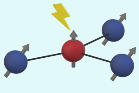
In a diamond crystal, three carbon atom nuclei (shown in blue) surround an empty spot called a nitrogen vacancy center, which behaves much like a single electron (shown in red). The carbon nuclei act as quantum bits, or qubits, and it turns out the primary source of noise that disturbs them comes from the jittery “electron” in the middle. By understanding the single source of that noise, it becomes easier to compensate for it, providing a key step toward quantum computing. This noise source can be accurately modeled, and suppressing its effects could have a major impact, as other sources of noise are relatively insignificant.

The team determined that the noise comes from one central defect, or one central electron that has a tendency to hop around at random. It jitters. That jitter, in turn, is felt by all those nearby nuclei, in a predictable way that can be corrected. The ability to apply this targeted correction in a successful way is the central breakthrough of this research.

The work so far is theoretical, but the team is actively working on a lab demonstration of this principle in action.

If the demonstration works as expected, this research could make up an important component of near and far term future quantum-based technologies of various kinds, including quantum computers and sensors.

______

Quantum Computing Breakthrough in Atom Control: 2020 study:

A team of scientists in Australia claim to have stumbled on a breakthrough discovery that will have “major implications” for the future of quantum computing. Describing the find as a “happy accident,” engineers at the University of New South Wales Sydney found a way to control the nucleus of an atom using electric fields rather than magnetic fields—which they have claimed could now open up a “treasure trove of discoveries and applications.”

Quantum computing expands on understandings of tech by basing research on quantum theory—analysing how energy works at atomic and subatomic levels. Electric fields make it easier to control the spin of atoms compared to magnetic fields, which are difficult to confine to small spaces as they have a “wide area of influence.” The study, published in Nature, solves a problem in finding a way to control nuclear spins with electricity, first suggested back in 1961 by the magnetic resonance expert and Nobel Laureate Nicolaas Bloembergen, the team said. “This discovery means that we now have a pathway to build quantum computers using single atom spins without the need for any oscillating magnetic field for their operation,” elaborated UNSW Scientia Professor of Quantum Engineering Andrea Morello. “Moreover, we can use these nuclei as exquisitely precise sensors of electric and magnetic fields, or to answer fundamental questions in quantum science. I have worked on spin resonance for 20 years of my life, but honestly, I had never heard of this idea of nuclear electric resonance” said Morello.

Researchers made a device containing an antimony atom and a special antenna, optimized to create a high-frequency magnetic field to control the nucleus of the atom. The experiment demands this field to be quite strong, so they applied a lot of power to the antenna. The test showed nuclear electric resonance is a “local microscopic phenomenon” and the electric field effectively distorted the atomic bonds around the nucleus, causing it to shift. Nuclear magnetic resonance is a technique used in a variety of scientific fields, such as medicine, chemistry and mining. The use of electric fields over magnetic fields could shake things up.

______

______

Companies developing quantum computing:

Companies currently developing quantum computers include IBM, Alibaba, Microsoft, Google, Intel, D-Wave Systems, Quantum Circuits, IonQ and Rigetti. Many of these firms work in conjunction with major university research teams, and all continue to accrue significant progress. The following provides an overview of the world of each of these pioneers in turn.

IBM:

IBM has been working to develop a quantum computer for over 35 years. It is also making significant progress, with several operational machines.  In 2016, IBM launched a website called the IBM Q Experience that made a 5 qubit quantum computer publicly available over the Internet. Since this time, this has been joined by a second 5 qubit machine and a 16 qubit machine, both of which are available for anybody to experiment with. To help those wishing to learn about and develop quantum computing, IBM offers an open source quantum computing software framework called Qiskit. In addition to the above, in November 2017 IBM announced that two 20 qubit machines were being added to its quantum cloud. These can be used by clients who are signed-up members of the IBM Q Network. This IBM describes as ‘a worldwide community of leading Fortune 500 companies, startups, academic institutions, and national research labs working with IBM to advance quantum computing and explore practical applications for business and science’. Also in November 2017, IBM announced that it had constructed a 50 qubit quantum processor, which remains its most powerful quantum hardware to date. In January 2019, IBM unveiled its IBM Q System One as the “world’s first integrated universal approximate quantum computing system designed for scientific and commercial use. This modular and relatively compact system is intended to be used outside of a laboratory environment.

Google:

Another tech giant that is working hard to make quantum computing a reality is Google, which operates its Quantum AI Laboratory. Google’s early with in quantum computing involved the use of a machine from Canadian pioneer D-Wave Systems. However, the company is now rapidly developing its own hardware, and in March 2018, announced a new 72 qubit quantum processor called ‘Bristlecone’. In June 2019, the director of Google’s Quantum Artificial Intelligence Lab, Hartmut Neven, revealed that the power of its quantum processors is now increasingly at a doubly exponential rate. This has been termed “Nevan’s Law”, and suggests that we may reach the point of quantum supremacy — where a quantum computer can outperform any classical computer — by the end of 2019. Indeed, in September 2019, a draft Google paper indicated that quantum supremacy had been achieved. This said, the jury is still out on whether this really the case.

Alibaba:

Over in China, the main web giant is Alibala, not Google. And in July 2015, Alibaba teamed up with the Chinese Academy of Sciences to form the ‘CAS – Alibaba Quantum Computing Laboratory’. As its Professor Jianwei Pan explained at the time, this has the mission to ‘undertake frontier research on systems that appear the most promising in realizing the practical applications of quantum computing . . . so as to break the bottlenecks of Moore’s Law and classical computing’. Like IBM, Alibaba has now made an experimental quantum computer available online. Specifically, in March 2018 the Chinese e-business giant launched its ‘superconducting quantum computing cloud’ to provide access to an 11 qubit quantum computer. This was developed with the Chinese Academy of Sciences, and allows users to run quantum programs and download the results.

Microsoft:

Microsoft is also keen to get in on the quantum computing action, and is working with some of the world’s top academics and universities to try and make this happen. To this end, Microsoft has set up several ‘Station Q’ labs, such as the one located at the University of California. In February 2019, Microsoft also announced the Microsoft Quantum Network to formalize its range of partnership coalitions. A key element of Microsoft’s strategy is the development of quantum computers based on ‘topological qubits’, which it believes will be less prone to errors (hence requiring fewer final system resources to be devoted to error correction). Microsoft also believes that topological qubits will be easier to scale to commercial application. Indeed, according to May 2018 article in Computer Weekly, Microsoft’s vice-president in charge of quantum computing believes that it could have commercial quantum computers on its Azure cloud platform just five years from now. On the software side, in December 2017 Microsoft released a preview of its quantum computing development kit. This is free to download, and includes a programming language called Q#, and a quantum computing simulator. In May 2019, Microsoft also reported that it is going to open source the development kit.

Intel:

As the world’s leading producer of microprocessors, Intel is working to develop quantum computing chips. To this end, it is also hedging its bets by taking two different research approaches. One of these strands is being conducted in conjunction with the leading Dutch quantum computing pioneer QuTech. In November 17, 2017 Intel announced the delivery of a 17 qubit test chip to its partner in the Netherlands. Then, in January 2018 at CES, it further announced the delivery of a 49 qubit test quantum processor called ‘Tangle Lake’. Intel’s second quantum computing research strand is taking place entirely inhouse, and involves the creation of processors based on a technology called ‘spin qubit’. This is a significant innovation, as spin qubit chips are manufactured using Intel’s traditional silicon fabrication methods. In June 2018, Intel reported that it had begun testing a 26 spin qubit chip. Already, the qubits on Intel’s spin qubit wafers are only about 50 nanometers across, or 1/1500th the width of a human hair. This means that, maybe a decade from now, Intel could be manufacturing tiny quantum processors containing thousands or millions of qubits. Unlike conventional CPUs, these would need to be supercooled to almost absolute zero. Intel in December 2019 unveiled what is believed to be a first of-its-kind cryogenic control chip — code-named Horse Ridge — that will speed up development of full stack quantum computing systems. According to Intel’s quantum computing web pages, the company is targeting production-level quantum computing within ten years, and anticipates that the technology will start to enter its “commercial phase” around 2025.

D-Wave Systems:

D-Wave Systems is a pure-play pioneer based in Canada, and way back in 2007 demonstrated a 16 qubit quantum computer. In 2011, it then sold a $10 million dollar, 128 qubit machine called the D-Wave One to Lockheed Martin. In 2013, D-Wave next sold a 512 Qubit D-Wave Two to NASA and Google. By 2015, D-Wave even broke the 1,000 qubit barrier with its D-Wave 2X, and in January 2017 sold its first 2,000 qubit D-Wave 2000Q to cyber security firm Temporal Defense Systems. However, notwithstanding all of the aforementioned milestones, D-Wave’s work remains controversial. This is because their hardware is based on an ‘adiabatic’ process called ‘quantum annealing’ that other pioneers have dismissed as ‘restrictive’ and ‘a dead end’. IBM, for example, uses a ‘gate-based’ approach to quantum computing that allows it to control qubits in a manner analogous to the manner in which a transistor controls the flow of electrons in a conventional microprocessor. But in a D-Wave system there is no such control.

D-wave is not nor does it pretend to be a general purpose quantum computer.  D-wave can instead solve a subset of quantum computing problems, known as quadratic unconstrained binary optimization, QUBO, quickly. Theoretically the class of QUBO problems where D-wave can outbeat classical computers is known to be those which are large, sparse, and not diagonally dominant. The class of practical problems where QUBO is appropriate is well known and includes certain problems such as protein folding, and quantum adiabatic simulation.  What D-Wave does is to use its hardware to solve optimization problems that can be expressed as ‘energy minimization problems’. This is indeed restrictive, but still allows the hardware to run certain algorithms far faster than a classical computer. In August 2016, a paper in Physical Review X reported that certain algorithms ran up to one hundred million times faster on a D-Wave 2X than on a single-core classical processor. One of the authors of this research also happened to be Google’s Director of Engineering. This all said, the jury remains out on the value of D-Wave’s work to the general development of quantum computing future.

The above noted, D-Wave continues to push forward significantly its variant of quantum computing. For example, in October 2018, it launched a cloud-based, quantum application environment called Leap. This provides real-time access to a D-Wave 2000Q quantum computer, and in March 2019 was expanded to provide access in Japan and across Europe.

In 2019, D-Wave announced a 5000 qubit system available mid-2020, using their new Pegasus chip with 15 connections per qubit.

Rigetti:

Another quantum computing pure-play is a start-up called Rigetti. The company already has over 120 employees, and has made a 19 qubit quantum computer available online through its developer environment called Forest.

Quantum Circuits:

Another quantum computing start-up is Quantum Circuits, which was established by leading quantum computing professor Robert Schoelkopf and other colleagues from Yale University. The company has raised $18 million of venture capital, and plans to beat the computing industry giants in the race to make a viable quantum computer.

IonQ:

The company is developing quantum computing based on a ‘trapped ions’ approach, which it argues ‘combines unmatched physical performance, perfect qubit replication, optical networkability, and highly-optimized algorithms’ in order to ‘create a quantum computer that is as scalable as it is powerful and that will support a broad array of applications across a variety of industries’.

AT&T:

The AT&T Foundry innovation center in Palo Alto, California has joined the California Institute of Technology to form the Alliance for Quantum Technologies (AQT). The Alliance aims to bring industry, government, and academia together to speed quantum technology development and emerging practical applications. This collaboration will also bring a research and development program named INQNET (INtelligent Quantum NEtworks and Technologies). The program will focus on the need for capacity and security in communications through future quantum networking technologies. Quantum networking will enable a new era of super-fast, secure networks. AT&T, through the AT&T Foundry, will help test relevant technologies for commercial applications.

Atos Quantum:

‘Atos Quantum’, the first quantum computing industry program in Europe, was announced in November 2016. Its aim is to anticipate the future of quantum computing and to be prepared for the opportunities and also the risks that come with it: opportunities such as superfast algorithms for database search, artificial intelligence or discovery of new pharmaceutical molecules – and risks such as the collapse of asymmetric cryptography. This global program aims to develop quantum computing solutions to understand the change in paradigm that quantum brings in the way algorithms are developed, but also to learn how to enhance cybersecurity products to anticipate quantum advantage and its impact on cryptography. Atos’ position as a leader in security and High-Performance Computing, together with its experience and expertise, provide a solid base from which to launch ‘Atos Quantum’. Atos’ ambition is to be a quantum player in two domains: quantum programming and simulation platforms and, later, next-generation quantum-powered supercomputers, as well as quantum-safe cybersecurity.

Accenture:

In response to predicted demand for quantum services, software companies are developing hardware-agnostic quantum platforms and applications. Accenture Labs is monitoring the quantum computing ecosystem and collaborating with leading companies such as Vancouver, Canada-based 1QBit. 1QBit is a software company dedicated to building development tools and software to solve the world’s most demanding computational challenges. The company’s platforms enable the development of hardware-agnostic applications that are compatible with both classical and quantum processors. Accenture and quantum software firm 1QBit collaborated with Biogen to develop a first-of-its-kind quantum-enabled molecular comparison application that could significantly improve advanced molecular design to speed up drug discovery for complex neurological conditions such as multiple sclerosis, Alzheimer’s, Parkinson’s and Lou Gehrig’s Disease.

Baidu:

Baidu has launched its own institute for quantum computing dedicated to the application of quantum computing software and information technology. The Baidu Quantum Computing Institute is headed by Professor Duan Runyao, director of the Centre for Quantum Software and Information at the University of Technology Sydney (UTS). During the launch, Professor Duan said that his plan is to make Baidu’s Quantum Computing Institute into a world-class institution within five years, according to local media. During the next five years, it will gradually integrate quantum computing into Baidu’s business. Duan will report directly to Baidu president Zhang Yaqin.

_____

Commercial availability of quantum computers:

The Canadian company D-Wave Systems currently sells a quantum computer named the D-Wave 2000Q, however, there are significant caveats with that offering. D-Wave advertises this system as having 2000 qubits, though differences in D-Wave’s definition of qubit relative to the rest of the quantum computing industry make this measurement not practically useful.  Further, the systems sold by D-Wave are designed specifically for quadratic unconstrained binary optimization, making them unsuitable for integer factorization required for cracking RSA encryption systems. Additionally, the D-Wave 2 (second-generation system) was found to not be faster than a traditional computer.

Likewise, Fujitsu offers a “quantum inspired” digital annealer, which is a traditional transistor-based computer designed for quantum annealing tasks, like D-Wave’s quantum computer. However, Fujitsu does not market this system as a true quantum computer, as the traditional transistor-based design allows it to operate at room temperature without requiring helium-based cooling solutions, as well as making it resistant to noise and environmental conditions which impact performance in quantum computers.

Quantum computing resources are widely available via cloud services, with vendor-specific frameworks. Presently, offerings are available from IBM Q (via Qiskit), while Google has introduced the Cirq framework, though it does not presently have a cloud offering in general availability. D-Wave Leap allows approved developers to conduct quantum experiments for free. Similarly, Fujitsu offers cloud access to their digital annealer system.

For buying systems outright, D-Wave’s 2000Q system costs $15 million (Notable buyers include Volkswagen Group and Virginia Tech.). A quantum computer is not something you are likely to find at your local big-box store. However, if your workloads are more general, building and buying a POWER9 deployment is likely a better value at present. Oak Ridge National Laboratory’s SUMMIT supercomputer is a POWER9 and NVIDIA Volta-driven system planned at 4600 nodes, with a computational performance in excess of 40 teraflops per node.

The CTO of Intel, Mike Mayberry, expects quantum technology to be commercialized within 10 years but IBM is aiming to make the technology mainstream within five years. Other experts believe a 15-year timeline is more realistic. Despite these predictions from some of the world’s biggest tech companies, there are also some experts, such as Gil Kalai, who believe practical quantum computing will never be achieved. However, it seems like most people involved in the field disagree with this opinion.

Google said in 2019 that its computer had performed a calculation in 200 seconds that would take the fastest supercomputers about 10,000 years. That claim was met with skepticism by IBM researchers, who said a classical computer that had a big enough hard drive could do it in 2.5 days. Even when that milestone is reached, the first quantum applications may be very specialized — that is, useful in certain kinds of mathematical problems that are important in chemistry or physics but little else. A so-called “universal” quantum computer is further off. The reason is errors, lots of them. Scientists have only been able to keep qubits in a quantum state for fractions of a second — in many cases, too short a period of time to run an entire algorithm. And as qubits fall out of a quantum state, errors creep into their calculations. These have to be corrected with the addition of yet more qubits, but this can consume so much computing power that it negates the advantage of using a quantum computer in the first place.

_______

_______

Quantum annealing:

Adiabatic quantum computation (AQC) is an alternative to the better-known gate model of quantum computation. The two models are polynomially equivalent, but otherwise quite dissimilar: one property that distinguishes AQC from the gate model is its analog nature. Quantum annealing (QA) describes a type of heuristic search algorithm that can be implemented to run in the ‘native instruction set’ of an AQC platform. D-Wave Systems Inc. manufactures quantum annealing processor chips that exploit quantum properties to realize QA computations in hardware. The chips form the centerpiece of a novel computing platform designed to solve optimization problems.

_

It’s important to keep in mind that quantum annealing algorithms in their basic form are remarkably similar to simulated annealing algorithms. Why? Because quantum tunneling strength plays the same role in quantum annealing as temperature does in simulated annealing. As time passes, the quantum tunneling strength in the quantum annealer drops dramatically, just as the temperature in the simulated annealer drops dramatically. It’s also easy to visualize the similarity between tunneling-strength and temperature. As time passes and quantum tunneling strength decreases, the system gets cozier and cozier with each progressively deeper valley in the energy landscape, and less and less inclined to tunnel its way out. Eventually, it gives up tunneling altogether when it finds itself (ideally) at the bottom of the deepest and coziest valley in the energy landscape (AKA the global minimum).

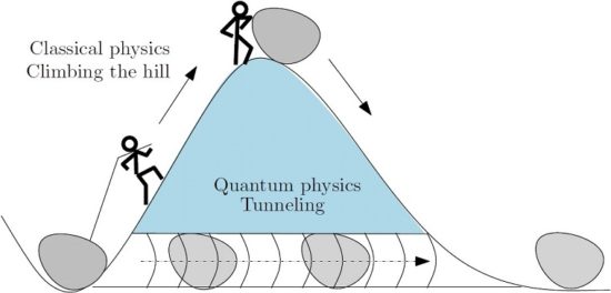
The first difference your bound to notice between relatively conventional quantum computers and quantum annealing computers is the number of qubits they use. While the state-of-the-art in conventional quantum computers is pushing a few dozen qubits in 2018, the leading quantum annealer has more than 2000 qubits. Of course, the trade-off is that quantum annealers are not universal but specialized quantum computers that technically tackle only optimization problems and sampling problems.

_

Quantum annealing is best for solving optimization problems. In other words, researchers are trying to find the best (most efficient) possible configuration among many possible combinations of variables. For example, Volkswagen (VW) recently conducted a quantum experiment to optimize traffic flows in the overcrowded city of Beijing, China. The experiment was run in partnership with Google and D-Wave Systems. The algorithm could successfully reduce traffic by choosing the ideal path for each vehicle, according to VW. Imagine applying this experiment on a global scale — optimizing every airline route, airport schedule, weather data, fuel costs, and passenger information, etc. for everyone, to get the most cost-efficient travel and logistics solutions. Classical computers would take thousands of years to compute the optimum solution to such a problem. Quantum computers, theoretically, can do it in a few hours or less, as the number of qubits per quantum computer increases.

Quantum annealing is the least powerful and most narrowly applied form of quantum computing. In fact, experts agree that today’s supercomputers can solve some optimization problems on par with today’s quantum annealing machines.

______

______

Quantum simulation:

Using quantum programs to model quantum systems themselves has vast potential for unlocking insights leading to innovations across many industries. Photosynthesis, superconductors, and complex molecules are examples of quantum systems that can be simulated using quantum programs.

Simulating microscopic systems that behave according to the laws of quantum mechanics is computationally expensive. We need to take into account all the possible states that can be in superposition and the number of states grows exponentially with the size of the system. In a quantum computer, we don’t need to model all of the states of the system. Instead, we embed the quantum state of the system that we want to simulate in the qubits of the computer itself, and run the simulation with a specific set of quantum gates. In other words, we use a quantum computer to simulate a quantum system.

Chemical molecules are quantum systems and therefore can be analyzed in this way. One such specific chemical is the nitrogenase enzyme, which, with a better understanding of its properties, could have the potential to reduce the energy consumption and greenhouse gas emission of current fertilizers.

Quantum chemistry is a branch of chemistry focused on the application of quantum mechanics in physical models and experiments of chemical systems. In particular, quantum simulation could be used to simulate protein folding — one of biochemistry’s toughest problems. Misfolded proteins can cause diseases like Alzheimer’s and Parkinson’s, and researchers testing new treatments must learn which drugs cause reactions for each protein through the use of random computer modeling. It is said that if a protein were to attain its correctly folded configuration by sequentially sampling all the possible drug-induced effects, it would require a time longer than the age of the universe to arrive at its correct natural state. A realistic mapping of the protein folding sequence would be a major scientific and healthcare breakthrough that could save lives. Quantum computers can help compute the vast number of possible protein folding sequences for making more effective medications. In the future, quantum simulations will enable rapid designer drug testing by accounting for every possible protein-to-drug combination.

Note:

Please differentiate between quantum simulator and quantum simulation.

Quantum simulator runs quantum algorithm on classical computer to simulate quantum mechanics on classical computer. Quantum simulation is run on quantum computer to exact computer model of a molecule or drug because quantum behaviour of electrons and atoms of such a molecule or drug is relatively close to the native behavior of a quantum computer.

______

______

Quantum supremacy:

In quantum computing, quantum supremacy is the goal of demonstrating that a programmable quantum device can solve a problem that classical computers practically cannot (irrespective of the usefulness of the problem). Physicists have been talking about the power of quantum computing for over 30 years, but the questions have always been: will it ever do something useful and is it worth investing in? For such large-scale endeavors it is good engineering practice to formulate decisive short-term goals that demonstrate whether the designs are going in the right direction. So, google researchers devised an experiment as an important milestone to help answer these questions.

Scientists at Google in October 2019 declared, via a paper in the journal Nature, that they’d done something extraordinary. In building a quantum computer that solved an incredibly hard problem in 200 seconds — a problem the world’s fastest supercomputer would take 10,000 years to solve — they’d achieved “quantum supremacy.” That is: Google’s quantum computer did something that no conventional computer could reasonably do.

Computer scientists have seen quantum supremacy — the moment when a quantum computer could perform an action a conventional computer couldn’t — as an elusive, important milestone for their field. There are many research groups working on quantum computers and applications, but it appears Google has beaten its rivals to this milestone.

The Sycamore Processor:

The quantum supremacy experiment was run on a fully programmable 54-qubit processor named “Sycamore.” It’s comprised of a two-dimensional grid where each qubit is connected to four other qubits. As a consequence, the chip has enough connectivity that the qubit states quickly interact throughout the entire processor, making the overall state impossible to emulate efficiently with a classical computer.

The success of the quantum supremacy experiment was due to improved two-qubit gates with enhanced parallelism that reliably achieve record performance, even when operating many gates simultaneously. Google achieved this performance using a new type of control knob that is able to turn off interactions between neighboring qubits. This greatly reduces the errors in such a multi-connected qubit system. They made further performance gains by optimizing the chip design to lower crosstalk, and by developing new control calibrations that avoid qubit defects.

According to John Preskill, the Caltech particle physicist who coined the term “quantum supremacy,” Google’s quantum computer ‘is something new in the exploration of nature. These systems are doing things that are unprecedented’.

Of note: Some researchers at IBM contest the “supremacy” claim, saying that a traditional supercomputer could solve the problem in 2.5 days, not 10,000 years. Still, 200 seconds is a lot quicker than 2.5 days. If the quantum computer isn’t supreme, it’s still extremely impressive because it’s so small and so efficient. “They got one little chip in the quantum computer and the supercomputer is covering a basketball court,” Preskill says.

However the much vaunted notion of quantum supremacy is more slippery than it seems. The image of a 50-qubit (or so) quantum computer outperforming a state-of-the-art supercomputer sounds alluring, but it leaves a lot of questions hanging. Outperforming for which problem? How do you know the quantum computer has got the right answer if you can’t check it with a tried-and-tested classical device? And how can you be sure that the classical machine wouldn’t do better if you could find the right algorithm?

_______

_______

Cybersecurity in quantum computing:

In a world where so much of our personal information is online, keeping our data—bank details or our medical records—secure is crucial. To keep it safe, our data is protected by encryption algorithms that the recipient needs to ‘unlock’ with a key. Prime number factoring is one method used to create encryption algorithms. The key is based on knowing the prime number factors of a large number. This sounds pretty basic, but it’s actually very difficult to figure out what the prime number factors of a large number are.

Classical computers can very easily multiply two prime numbers to find their product. But their only option when performing the operation in reverse is a repetitive process of checking one number after another. Even performing billions of calculations per second, this can take an extremely long time when the numbers get especially large. Once numbers reach over 1000 digits, figuring out its prime number factors is generally considered to take too long for a classical computer to calculate—the data encryption is ‘uncrackable’ and our data is kept safe and sound.

Nobody wants to factor very large numbers! That’s because it’s so difficult – even for the best computers in the world today. In fact, the difficulty of factoring big numbers is the basis for much of our present day cryptography. It’s based on math problems that are too tough to solve. RSA encryption, the method used to encrypt your credit card number when you’re shopping online, relies completely on the factoring problem. The website you want to purchase from gives you a large “public” key (which anyone can access) to encode your credit card information. This key actually is the product of two very large prime numbers, known only to the seller. The only way anyone could intercept your information is to know those two prime numbers that multiply to create the key. Since factoring is very hard, no eavesdropper will be able to access your credit card number and your bank account is safe. Unless, that is, somebody has built a quantum computer and is running Peter Shor’s algorithm!  In 1994, mathematician Peter Shor came up with an algorithm that would enable quantum computers to factor large prime numbers significantly faster than by classical methods. As quantum computing advances we may need to change the way we secure our data so that quantum computers can’t access it.

_

How security is quantified:

The security of cryptography relies on certain “hard” problems—calculations that are practical to do with the right cryptographic key, but impractically difficult to do without it. A “hard” problem should take the best computers available billions of years to solve; an “easy” problem is one that can be solved very quickly.  The most widely used Public-key cryptography (PKC) systems, including RSA, Diffie-Hellman, and ECDSA, rely on the intractability of integer factorization and discrete log problems. These problems are hard for classical computers to solve, but easy for quantum. This means that as soon as a large-scale universal quantum computer is built, you will not be able to rely on the security of any scheme based on these problems.

To quantify the security of cryptosystems, “bits of security” are used. You can think of this as a function of the number of steps needed to crack a system by the most efficient attack. A system with 112 bits of security would take 2¹¹² steps to crack, which would take the best computers available today billions of years. Algorithms approved by NIST provide at least 112 bits of security. The security of encryption depends on the length of the key and the cryptosystem used.

Shor’s algorithm will be able to crack PKC systems like RSA and Diffie-Hellman; Grover’s will reduce the security of symmetric cryptosystems like the Advanced Encryption Standard (AES), but not as drastically.

_

Table below compares the security of both classical computers and quantum computers provided by AES and RSA.

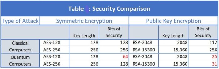
AES-128 and RSA-2048 both provide adequate security against classical attacks, but not against quantum attacks. Doubling the AES key length to 256 results in an acceptable 128 bits of security, while increasing the RSA key by more than a factor of 7.5 has little effect against quantum attacks.

The hash function SHA-256 is quantum-safe, which means that there is no efficient known algorithm, classical or quantum, which can invert it. While there is a known quantum algorithm, Grover’s algorithm, which performs “quantum search” over a black-box function, SHA-256 has proven to be secure against both collision and preimage attacks. In fact, Grover’s algorithm can only reduce 𝑁 queries of the black-box function, SHA in this case, to √N, so instead of searching 2²⁵⁶ possibilities, we only have to search 2¹²⁸, which is even slower than algorithms like van Oorschot–Wiener algorithm for generic collision search and Oechslin’s rainbow tables for generic pre-image search on classical computers.

_

The development of large quantum computers, along with the extra computational power it will bring, could have dire consequences for cyber security. For example, it is known that important problems such as factoring and the discrete log, problems whose presumed hardness ensures the security of many widely used protocols (for example, RSA, DSA, ECDSA), can be solved efficiently (and the cryptosystems broken), if a quantum computer that is sufficiently large, “fault tolerant” and universal, is developed.

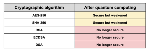
While this theoretical result has been known since the 1990s, the actual prospect of building such a device has only recently become realistic (in medium term). However, addressing the eminent risk that adversaries equipped with quantum technologies pose is not the only issue in cyber security where quantum technologies are bound to play a role.

_

Quantum cyber security is the field that studies all aspects affecting the security and privacy of communications and computations caused by the development of quantum technologies.

Quantum technologies may have a negative effect to cyber security, when viewed as a resource for adversaries, but can also have a positive effect, when honest parties use these technologies to their advantage. The research can, broadly speaking, be divided into three categories that depend on who has access to quantum technologies and how developed these technologies are (see figure below). In the first category we ensure that currently possible tasks remain secure, while in the other two categories we explore the new possibilities that quantum technologies bring.

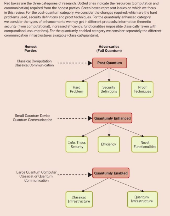
Figure above shows schematic representation of the quantum cyber security research landscape.

As is typical in cryptography, we first assume the worst-case scenario in terms of resources, where the honest parties are fully classical (no quantum abilities), while the adversaries have access to any quantum technology (whether this technology exists currently or not). In particular we assume they have a large quantum computer. Ensuring the security and privacy guarantees of a classical protocol remain intact is known as post-quantum (or “quantum-safe”) security.

In the second category we allow honest parties to have access to quantum technologies in order to achieve enhanced properties, but we restrict this access to those quantum technologies that are currently available (or that can be built in near-term). Requesting this level of quantum abilities comes from the practical demand to be able to construct now, small quantum devices/gadgets that implement the “quantum” steps of (the honest) protocols. The adversaries, again, can use any quantum technology. In this category we focus on achieving classical functionalities but we are able to enhance the security or efficiency of the protocols beyond what is possible classically by using current state-of-the-art quantum gadgets.

Finally, the third category looks further in the future and examines the security and privacy of protocols that are possible (are enabled) by the existence of quantum computers. We assume there exist quantum computation devices that offer advantages in many useful applications compared with the best classical computers. At that time, there will be tasks that involve quantum computers and communication and processing of quantum information, where the parties involved want to maintain the privacy of their data and have guarantees on the security of the tasks achieved. This period may not be too far, since quantum devices being developed now are already crossing the limit of quantum computations that can be simulated by classical supercomputers.

These categories, in general, include all aspects of cyber security.

__

Quantum computers threaten Blockchain security:

The Blockchain is a digital tool based on cryptography techniques that protects information from unauthorized changes. It lies at the root of the Bitcoin cryptocurrency. Blockchain-related products are also used everywhere from finance to manufacturing and healthcare in a market currently worth over 150 billion USD. The Blockchain is a secure digital record or ledger. It is maintained by users around the globe, rather than a central administration. Decisions, such as whether to add an entry (or block), are based on consensus – so personal trust doesn’t come into it. A network of computer centers performs powerful calculations to verify entries and assign a unique number, or hash, to blocks. Any party, inside or outside the network, is able to check the integrity of the ledger by means of a simple calculation. By 2025, analysts predict that up to ten percent of global GDP will be stored on blockchains. Blockchain networks including Bitcoin’s architecture relies on two algorithms: Elliptic Curve Digital Signature Algorithm (ECDSA) for digital signatures and SHA-256 as a hash function.

One-way codes:

Blockchain security relies on ‘one-way’ mathematical functions. These are straightforward to run on a conventional computer but difficult to calculate in reverse. For example, multiplying two large prime numbers is easy, but finding the prime factors of a given product is hard. Such functions are used to generate digital signatures that blockchain users cite to authenticate themselves to others. These are easy to check but extremely hard to forge. One-way functions are also used to validate the history of transactions in the blockchain ledger. The hash, a short sequence of bits, is derived from a combination of the existing ledger and the block that is to be added; this alters whenever contents are changed. Again, it is relatively easy to find the hash of a block (to process information to add a record) but difficult to pick a block that would yield a specific hash value (reversing the process to derive the information that generated the hash).

Bitcoin also requires that the hash meets a mathematical condition. Anyone who wishes to add a block to the ledger must keep their computer running a random search until the condition is reached. This process slows the addition of blocks to the network, giving time for everything to be recorded and checked by everyone. It also prevents any individual from monopolizing the administration of the network, because anyone with sufficient computational power can contribute blocks.

Yet within a decade, quantum computers will be able to calculate one-way functions currently used to secure the internet and financial transactions, including blockchains. Widely deployed one-way encryption will instantly become obsolete.

Quantum Threat to Blockchains: Shor’s and Grover’s Algorithms:

Quantum computers take advantage of physical effects like superpositions of states and entanglement to perform computational tasks. To date, they are still much less powerful than conventional computers. But within few years quantum devices will emerge that are capable of outperforming computers on certain tasks. Breaking security protocols based on cryptographic algorithms is one of them.  A blockchain is secured by two major mechanisms: 1) encryption via asymmetric cryptography and 2) hashing.

_

How true quantum computer could challenge asymmetric cryptography and hashing?

1. Shor’s Algorithm and its challenge to Asymmetric Cryptography:

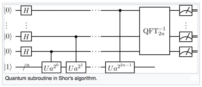
The public and private keys used to secure blockchain transactions are both very large numbers, hashed into a group of smaller numbers. Asymmetric cryptography algorithms depend on computers being unable to find the prime factors of these enormous numbers.

Shor’s Algorithm is a conceptual quantum computer algorithm optimized to solve for prime factors. It takes a factor (a number), n, and outputs its factors. Its magic lies in reducing the number of steps necessary to find a number’s prime factors (thereby potentially cracking public and private keys).

The algorithm is broken up into two parts:

-1. A reduction of the factoring problem to the problem of order-finding (which can be performed today on a classical computer)

-2. A quantum algorithm to solve the order-finding problem (which is ineffective today due to the lack of quantum computing capabilities)

Using the most common encryption standard, it takes a classical computer 2¹²⁸, that is to say 340,282,366,920,938,463,463,374,607,431,768,211,456 basic operations, to find the private key associated with a public key. On a quantum computer, it would take 128³ (i.e. only 2,097,152) basic operations to find the private key associated with a public key.

This is why conceptually the development of true quantum computing could pose a threat to today’s blockchain encryption. Of course, this threat is yet to materialize. Today, due to the lack of development in quantum computing, Shor’s Algorithm cannot be used in any serious way.

_

2. Grover’s Algorithm and its challenge to Hashing:

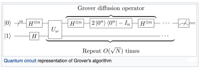
Cryptographic hashing is much harder for a potential quantum computer to crack (compared to asymmetric cryptography). However, there is also a quantum algorithm that could potentially make it significantly easier (but still very difficult) to break cryptographic hashing. Grover’s Algorithm allows a user to search through an unordered list for specific items. Grover’s Algorithm is probabilistic: it gauges the probabilities of various potential states of the system.

Here’s how it works:

Imagine being given an unordered list of a certain number of elements and asked to find the element among them that satisfies a certain condition. You could use a classical computer to go through each element to find the one that satisfies the condition. However, quantum computing uses superposition to test multiple inputs simultaneously. A quantum computer would use Grover’s Algorithm to conduct several rounds of computation. Through each round of computation, the probability of certain items having the desired condition increases. The algorithm narrows down selections as it progresses, and spits out one high probability result at the end.

You would require 2²⁵⁶ (which is a 78 digit number) of basic operations with a classical computer to find the correct hash. For a quantum computer using Grover’s Algorithm, it would only take 2¹²⁸ (which a 39 digit number) of basic operations to solve for the correct hash.

_

In a nutshell:

If true, powerful quantum computers existed today, they would likely pose a serious threat to asymmetric encryption but not to hashing. They could use Shor’s Algorithm to significantly reduce the number of steps to factor big numbers, thus more easily revealing the private key associated with a given public key. They could also use Grover’s Algorithm to attempt to break cryptographic hashing more easily than a classical computer can today, but this task would still be next to impossible. Luckily, given the primitive state of quantum computing today, we cannot expect any serious challenge to blockchain security mechanisms from either of these algorithms.

_____

McAfee: Start protecting against quantum computing hacks now: February 2020:

McAfee’s chief technology officer warned that it’s time for companies to start worrying about quantum computing attacks that can break common forms of encryption available today, even if quantum computing isn’t going to be practical for a while. Steve Grobman, CTO of the cybersecurity firm, made the remarks in a keynote address at RSA, the big security conference in San Francisco recently.

Cloud computing is sweeping through the industry, and it will enable the use of quantum computing. And that’s a problem, as quantum computers may be able to break encryption techniques such as RSA encryption much faster than traditional computers can. Typically, encryption techniques make it easy to encode data but hugely difficult to decode it without the use of a special key. The security is possible only because of the huge amount of time it takes for a classical computer to do the computations. If the quantum computing speeds up dramatically and arrives sooner than expected at practical prices, then the safety of today’s encryption techniques will be compromised, Grobman said.

Grobman said cybercriminals can siphon off data today and unlock it when quantum cryptoanalysis becomes practical. So companies have to consider the sensitivity of their data and how long it must be protected. For names matched to social security numbers, that’s a long time, as an example. “We need quantum-resistant algorithms as soon as possible,” Grobman said.

_

Criminals are unlikely to be able to afford to purchase or run quantum computers in near future, but nation-states are another matter. Given how badly the US is losing the cyber war to Russia, it’s no surprise Russia is at the forefront of quantum computer research. Should the Russian government break all of American encryption before the US develops countermeasures, election interferences will seem like small potatoes.

______

Quantum-safe cryptography:

_

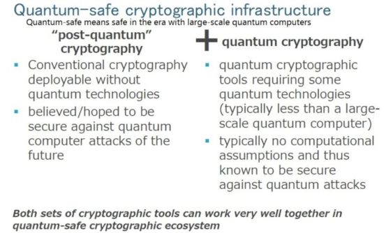
Post-quantum cryptography:

Quantum computers may become a technological reality; it is therefore important to study cryptographic schemes used against adversaries with access to a quantum computer. The study of such schemes is often referred to as post-quantum cryptography. The need for post-quantum cryptography arises from the fact that many popular encryption and signature schemes (schemes based on ECC and RSA) can be broken using Shor’s algorithm for factoring and computing discrete logarithms on a quantum computer. Examples for schemes that are, as of today’s knowledge, secure against quantum adversaries are McEliece and lattice-based schemes, as well as most symmetric-key algorithms. Surveys of post-quantum cryptography are available.

There is also research into how existing cryptographic techniques have to be modified to be able to cope with quantum adversaries. For example, when trying to develop zero-knowledge proof systems that are secure against quantum adversaries, new techniques need to be used: In a classical setting, the analysis of a zero-knowledge proof system usually involves “rewinding”, a technique that makes it necessary to copy the internal state of the adversary. In a quantum setting, copying a state is not always possible (no-cloning theorem); a variant of the rewinding technique has to be used.

Post quantum algorithms are also called “quantum resistant”, because – unlike quantum key distribution – it is not known or provable that there will not be potential future quantum attacks against them. Even though they are not vulnerable to Shor’s algorithm, the NSA is announcing plans to transition to quantum resistant algorithms. The National Institute of Standards and Technology (NIST) believes that it is time to think of quantum-safe primitives.

Post-quantum public-key algorithms:

At this stage, five main approaches for public-key algorithms are thought to be resistant to quantum-computing attacks. These are hash-based cryptography, lattice-based cryptography, supersingular elliptic-curve isogeny cryptography, multivariate cryptography, and code-based cryptography.

Research into their security and usability is ongoing, but it is hoped that at least one option based on these techniques will be suitable for the post-quantum cryptographic world.

_

Quantum cryptography:

Post-quantum cryptography is distinct from quantum cryptography, which refers to using quantum phenomena to achieve secrecy and detect eavesdropping.

At this stage of the article, you might be beginning to think that quantum computing is all bad news when it comes to internet security and cryptography. Despite the complications that quantum computing may bring to these fields, there could also be some benefits.

Quantum cryptography is different from traditional cryptographic systems in that it relies more on physics, rather than mathematics, as a key aspect of its security model. Essentially, quantum cryptography is based on the usage of individual particles/waves of light (photon) and their intrinsic quantum properties to develop an unbreakable cryptosystem (because it is impossible to measure the quantum state of any system without disturbing that system.) Quantum cryptography uses photons to transmit a key. Once the key is transmitted, coding and encoding using the normal secret-key method can take place.

The unique properties of quantum mechanics open up a world of new opportunities when it comes to secure communication. Some of these, such as quantum key-distribution, are already being used. Potential quantum mechanisms for the future include Kak’s three stage protocol and quantum digital-signatures, among other possibilities.

Quantum key distribution:

Quantum key distribution is much like any other key exchange protocol. It allows two parties to securely establish a symmetric key which they can use to encrypt their future communications. The main difference is that it leverages the unique properties of quantum mechanics, allowing the two parties to detect if an attacker is eavesdropping on the messages. This is made possible because of one of the fundamental principles of quantum mechanics: Any attempt to measure a quantum system will alter it. Since intercepting data is, in essence, a form of measurement, a quantum key-distribution scheme will detect any anomalies that come from an attacker eavesdropping and abort the connection. If the system does not detect any eavesdropping, the connection will proceed, and the parties can be certain that the key they have developed is secure, as long as adequate authentication has taken place.

The most well-known and developed application of quantum cryptography is quantum key distribution (QKD). QKD describes the use of quantum mechanical effects to perform cryptographic tasks or to break cryptographic systems. QKD involves sending encrypted data as classical bits over networks, while the keys to decrypt the information are encoded and transmitted in a quantum state using qubits. Various approaches, or protocols, have been developed for implementing QKD. A widely used one known as BB84. The principle of operation of a QKD system is quite straightforward: two parties (Alice and Bob) use single photons that are randomly polarized to states representing ones and zeroes to transmit a series of random number sequences that are used as keys in cryptographic communications. Both stations are linked together with a quantum channel and a classical channel. Alice generates a random stream of qubits that are sent over the quantum channel. Upon reception of the stream Bob and Alice — using the classical channel — perform classical operations to check if an eavesdropper has tried to extract information on the qubits stream. The presence of an eavesdropper is revealed by the imperfect correlation between the two lists of bits obtained after the transmission of qubits between the emitter and the receiver. One important component of virtually all proper encryption schemes is true randomness which can elegantly be generated by means of quantum optics. In a typical QKD set-up, the photons are generated by a single photon source, encoded into binary values (i.e., representing “0” and “1”) and then transmitted to the receiver either via optical fibers or in free space. The receiver then decodes the state of photons and detects them using single photon sensitive detectors and time-tagging electronics.

Quantum key-distribution is currently used in certain situations where the need for security is high, such as banking and voting. We’re already starting to see more QKD networks emerge. The longest is in China, which boasts a 2,032-kilometer (1,263-mile) ground link between Beijing and Shanghai. Banks and other financial companies are already using it to transmit data. In the US, a startup called Quantum Xchange has struck a deal giving it access to 500 miles (805 kilometers) of fiber-optic cable running along the East Coast to create a QKD network. The initial leg will link Manhattan with New Jersey, where many banks have large data centers. Although QKD is relatively secure, it would be even safer if it could count on quantum repeaters. It is still relatively expensive and cannot be used over large distances, which has prevented further adoption.

Kak’s three-stage protocol:

Subhash Kak’s three-stage protocol is a proposed mechanism for using quantum cryptography to encrypt data. It requires the two parties in the connection to first be authenticated, but can theoretically provide a way to continuously encrypt data in a way that is unbreakable.

Although it could be used to establish keys, it differs from quantum key-distribution because it can also be used to encrypt the data. Quantum key-distribution only uses quantum properties to establish the key–the data itself is encrypted using classical cryptography.

Kak’s three-stage protocol relies on random polarization rotations of photons. This method allows the two parties to securely send data over an unsafe channel. The analogy that is usually used to describe the structure is to picture two people, Alice and Bob. Alice has a secret that she wants to send to Bob, but she does not have a safe communication channel over which to do so. To securely send her secret over an insecure channel, Alice puts her secret in a box, then locks the box with a chain around the outside. She then sends the box to Bob, who locks the box with his own chain as well. Bob then sends the box back to Alice, who takes off her lock. She then returns the box to Bob. Since the box now only has Bob’s lock protecting it, he can unlock it and access the secret data.

This method allows Alice to send Bob a secret without any third party being able to access it. This is because the box has at least one person’s lock on it each time it is sent across the insecure channel.

Quantum digital signatures:

Quantum computing threatens our commonly used digital signature schemes, since they rely on public-key ciphers that are vulnerable to Shor’s algorithm. However, the new technology also opens the door to quantum digital signatures, which would be resistant to these attacks.

Quantum digital signatures would work just like normal digital signatures, and could authenticate data, check its integrity and provide non-repudiation. The difference is that they would rely on the properties of quantum mechanics, rather than on mathematical problems that are difficult to reverse, which is what the systems we currently use are based on.

There are two different approaches to quantum digital signatures:

• A classical bit string is used for the private key, and a public quantum key is derived from it.
• A quantum bit string is used for the private key, and a public quantum key is derived from it.

Both of these types of quantum digital signatures differ from classical digital signatures, because they use one-way quantum functions. These functions would be impossible to reverse, while classical one-way functions are just incredibly difficult to reverse.

_

Cybersecurity of quantum computer:

This is more of a placeholder. Quantum computers are very isolated and they store no data, so they have a minimal security footprint. They do have network access for submitting programs for execution remotely, but that’s a classical computer connected to the network as a front end, not the quantum computer itself. The hybrid mode of operation does have a security component, but once again this is actually a classical computer front end which then interfaces directly to the quantum computer.

Although the emerging field of quantum cryptography is quite exciting, quantum computers as currently envisioned don’t have any real role in encryption. Quantum communication is another story, with flying qubits, but has nothing to do with operation on stationary qubits using quantum logic gates.

_

There is no need to worry today:

Although there is plenty of chatter about post-quantum cryptography and the prospect of a quantum computer being able to break even strong public cryptography keys, that’s not a reality today or the near future.

Prime factorization (technically integer factorization of a bi-prime or semiprime — factoring a large integer into exactly two factors which are each a large prime number), the required calculation to break encryption keys, is still a young and emerging area of research for quantum computing. A quantum computer could use Shor’s algorithm to get your private from your public key, but the most optimistic scientific estimates say that even if this were possible, it won’t happen during this decade.

A 160-bit elliptic curve cryptographic key could be broken on a quantum computer using around 1000 logical qubits while factoring the security-wise equivalent 1024-bit RSA modulus would require 2000 logical qubits. And to implement Shor’s algorithm for factoring a 2048 bit number we need more than 4000 logical qubits and billions of physical qubits. however, Google’s Craig Gidney and KTH’s Martin Ekera demonstrated that a quantum system could crack 2,048-bit RSA encryption with just 20 million quantum bits (qubits), rather than requiring 1 billion qubits as previously theorized, in only eight hours with this technique. By comparison, Google’s measly 53 qubits are still no match for this kind of cryptography. But that isn’t to say that there’s no cause for alarm, the fact is that the rate of advancements in quantum technology is increasing, and that could, in time, pose a threat. Sure, better prime factorization is coming, but not so rapidly as to be worthy of any great alarm today.

_______

_______

Quantum computing, AI and machine learning:

_

Basics:

Machine Learning: is how computers learn patterns in data.

Quantum Computing: is the use of quantum mechanical phenomena such as superposition and entanglement to perform computation. A quantum computer is used to perform such computation, which can be implemented theoretically or physically.

Quantum Machine Learning: is about how quantum computers and other quantum information processors can learn patterns in data that cannot be learned by classical machine learning algorithms.

_

The term Artificial intelligence (AI) is used fairly broadly these days; however, AI is a distilled concept that machines will be able to execute tasks characteristic of human intelligence. Machine Learning (ML) at its core is a simple way of achieving AI, and AI/ML can offer assistance in speeding up and parsing extremely large chunks of data whilst creating and analyzing predictive models and trends that will help unravel patterns not easily determined by us. Machine learning is a faster way of determining and analyzing these patterns (rather than using traditionally-coded algorithms) and can be used for a number of different applications, however, its application in AI is the one that’s got the whole world abuzz. Quantum computation researchers hope to find more quantum algorithms demonstrating significant speedup over classical algorithms. They are looking for new problems suited to this purpose, and some AI problems seems to be good candidates. On the other hand, the AI community believes that quantum computation shows significant potential for solutions to currently intractable problems.

_

Roughly speaking, AI has two overall goals: (1) engineering goal – to develop intelligent machines; and (2) scientific goal – to understand intelligent behaviors of humans, animals and machines. AI researchers mainly employ computing techniques to achieve both the engineering and scientific goals. Indeed, “computational intelligence” is a more suitable name of the subject of AI to highlight the key role played by computers in AI. Naturally, the rapid development of quantum computation leads us to ask the question: how can this new computing technique help us in achieving the goals of AI. It seems obvious that quantum computation will largely contribute to the engineering goal of AI by applying it in various AI systems to speed up the computational process, but it is indeed very difficult to design quantum algorithms for solving certain AI problems that are more efficient than the existing classical algorithms for the same purpose. At this moment, it is also not clear how quantum computation can be used in achieving the scientific goal of AI. Instead, it is surprising that quite a large amount of literature is devoted to applications of quantum theory in AI and vice versa, not through quantum computation. Research arising from the interplay between quantum theory and AI can be roughly classified into two categories: (1) Using some ideas from quantum theory to solve certain problems in AI; and (2) Conversely, applying some ideas developed in AI to quantum theory. It can be observed from the existing works that due to its inherent probabilistic nature, quantum theory can be connected to numerical AI in a more spontaneous way than to logical AI.

__

The intersection of machine learning and quantum computing:

Quantum computing has the possibility to make machine learning AI solutions exponentially faster at crunching their datasets than their traditional computing counterparts — although you can’t code these ML/AI algorithms in the traditional sense. However, the intersection of these two fields goes even further than that, and it’s not just AI applications that can benefit. There is an intersecting area where quantum computers implement machine learning algorithms and traditional machine learning methods are employed to assess the quantum computers. This area of research is developing at such blazing speeds that it has spawned an entire new field called Quantum Machine Learning (QML). Recent work has produced quantum algorithms that could act as the building blocks of machine learning programs, but the hardware and software challenges are still considerable and the development of fully functional quantum computers is still far off.

There are 4 approaches to machine learning, categorised by whether the system under study is classic or quantum, and whether the information processing device is classical or quantum as seen in the figure below:

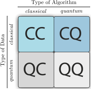
Figure above shows four different approaches to combine the disciplines of quantum computing and machine learning. The first letter refers to whether the system under study is classical or quantum, while the second letter defines whether a classical or quantum information processing device is used.

_

Quantum artificial intelligence:

Quantum artificial intelligence (QAI) is an interdisciplinary field that focuses on building quantum algorithms for improving computational tasks within artificial intelligence, including sub-fields like machine learning. Quantum mechanics phenomena, superposition and entanglement, are allowing quantum computing to perform computations which are much more efficient than classical AI algorithms used in computer vision, natural language processing and robotics. The entire concept of quantum-enhanced AI algorithms is still in conceptual research domain. Building on recent theoretical proposals, initial practical studies suggest that these concepts have the possibility to be implemented in the laboratory, under strictly controlled conditions.

_

Quantum machine learning (QML):

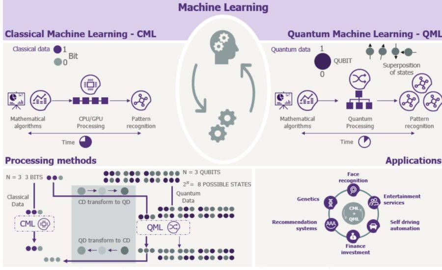
Quantum machine learning is an emerging interdisciplinary research area at the intersection of quantum physics and machine learning. The most common use of the term refers to machine learning algorithms for the analysis of classical data executed on a quantum computer, i.e. quantum-enhanced machine learning. While machine learning algorithms are used to compute immense quantities of data, quantum machine learning increases such capabilities intelligently, by creating opportunities to conduct analysis on quantum states and systems. This includes hybrid methods that involve both classical and quantum processing, where computationally difficult subroutines are outsourced to a quantum device. These routines can be more complex in nature and executed faster with the assistance of quantum devices. Furthermore, quantum algorithms can be used to analyze quantum states instead of classical data.  Beyond quantum computing, the term “quantum machine learning” is often associated with classical machine learning methods applied to data generated from quantum experiments (i.e. machine learning of quantum systems), such as learning quantum phase transitions or creating new quantum experiments.  Quantum machine learning also extends to a branch of research that explores methodological and structural similarities between certain physical systems and learning systems, in particular neural networks. For example, some mathematical and numerical techniques from quantum physics are applicable to classical deep learning and vice versa. Finally, researchers investigate more abstract notions of learning theory with respect to quantum information, sometimes referred to as “quantum learning theory”.

_

Machine learning with quantum computers:

Quantum-enhanced machine learning refers to quantum algorithms that solve tasks in machine learning, thereby improving and often expediting classical machine learning techniques. Such algorithms typically require one to encode the given classical data set into a quantum computer to make it accessible for quantum information processing. Subsequently, quantum information processing routines are applied and the result of the quantum computation is read out by measuring the quantum system. For example, the outcome of the measurement of a qubit reveals the result of a binary classification task. While many proposals of quantum machine learning algorithms are still purely theoretical and require a full-scale universal quantum computer to be tested, others have been implemented on small-scale or special purpose quantum devices.

_

Quantum neural networks:

Quantum analogues or generalizations of classical neural nets are often referred to as quantum neural networks. The term is claimed by a wide range of approaches, including the implementation and extension of neural networks using photons, layered variational circuits or quantum Ising-type models. Quantum neural networks are often defined as an expansion on Deutsch’s model of a quantum computational network. Within this model, nonlinear and irreversible gates, dissimilar to the Hamiltonian operator, are deployed to speculate the given data set. Such gates make certain phases unable to be observed and generate specific oscillations. Quantum neural networks apply the principals quantum information and quantum computation to classical neurocomputing. Current research shows that QNN can exponentially increase the amount of computing power and the degrees of freedom for a computer, which is limited for a classical computer to its size. A quantum neural network has computational capabilities to decrease the number of steps, qubits used, and computation time. The wave function in quantum mechanics is the neuron for neural networks.

_

Limits and discoveries in Quantum Deep Learning:

1. Main obstacles limiting quantum growth in the deep learning area

-The first obstacle to quantum neural networks was the lack of a real quantum computer to experiment with

-The second obstacle was the impossibility of training quantum networks

-The third problem, that the classic neuron/perceptron has nonlinear functions, putting it in conflict with the quantum qubits that operate only with unity and linearity

2. Main discoveries have changed these obstacles

-Recently several companies have delivered quantum computers in the last year, including IBM, who has made theirs available to researchers for free over the Internet

-A new algorithm now solves that problem using two main steps: Simple Quantum Neural Network and Quantum Neural Network training

-This issue has been solved with a new quantum perceptron using a special quantum circuit, the Repeat-Until-Success (RUS) circuit

_

The use of quantum algorithms in artificial intelligence techniques will boost machines’ learning abilities. This will lead to improvements in the development, among others, of predication systems, including those of the financial industry. However, we’ll have to wait to start these improvements being rolled out. The processing power required to extract value from the unmanageable swaths of data currently being collected, and especially to apply artificial intelligence techniques such as machine learning, keeps increasing.

Researchers have been trying to figure out a way to expedite these processes applying quantum computing algorithms to artificial intelligence techniques, giving rise in the process to a new discipline that’s been dubbed Quantum Machine Learning (QML). Quantum machine learning can be more efficient than classic machine learning, at least for certain models that are intrinsically hard to learn using conventional computers.  Machine learning and artificial intelligence technologies are the two key areas of research in the application of quantum computing algorithms. One of the particularities of this calculation system is that it allows representing several states at the same time, which is particularly convenient when using AI techniques. For example, as noted by Intel, voice-assistants could greatly benefit from this implementation, as quantum could exponentially help improve their accuracy, boosting both their processing power and the amount of data they would be able to handle.  Quantum computing increases the number of calculation variables machines can juggle and therefore allow them to provide faster answers, much like a person would.

More accurate algorithms:

The ability to represent and handle so many states makes quantum computing extremely adequate for solving problems in a variety of fields. Intel has opened several lines of research on quantum algorithms. The first applications they are going to see are in fields such as material sciences, where the modeling of small molecules is a computing intensive task. Going forward, larger machines will allow designing medicines or optimizing logistics to, for example, find the most efficient route among any number of alternatives. Currently, most industrial applications of artificial intelligence come from the so-called supervised learning, used in tasks such as image recognition or consumption forecasting. In this area, based on the different QML proposals that have already been set forth, it is likely that we’ll start seeing acceleration – which, in some cases, could be exponential – in some of the most popular algorithms in the field, such as ‘support vector machines’ and certain types of neural networks.

A less-treaded path, but which shows great promise, is the field of non-supervised learning. Dimensionality reduction algorithms are a particular case. These algorithms are used to represent our original data in a more limited space, but preserving most of the properties of the original dataset. In this point, the researcher notes the use of quantum computing will come in particularly handy at the time of pinpointing certain global properties in a dataset, not so much specific details.

Applications in the banking sector:

In the financial sector, the combination of AI with quantum computing may help improve and combat fraud detection. On the one hand, models trained using a quantum computer could be capable of detecting patterns that are hard to spot using conventional equipment. At the same time, the acceleration of algorithms would yield great advantages in terms of the volume of information that the machines would be able to handle for this purpose. Work is also being conducted in developing models that will allow to combine numerical calculations with expert advice to make final financial decisions. One of the main advantages is that these models are easier to interpret than neural network algorithms, and therefore more likely to earn regulatory approval.  Also, one of the hottest trends in banking right now is providing customers with tailored products and services using advanced recommendation systems. In this sense, several quantum models have already been proposed aimed at enhancing these systems’ performance.

_

Artificial intelligence controls quantum computers, a 2018 study:

Summary: Researchers present a quantum error correction system that is capable of learning thanks to artificial intelligence.

The basis for quantum information is the quantum bit, or qubit. Unlike conventional digital bits, a qubit can adopt not only the two states zero and one, but also superpositions of both states. In a quantum computer’s processor, there are even multiple qubits superimposed as part of a joint state. This entanglement explains the tremendous processing power of quantum computers when it comes to solving certain complex tasks at which conventional computers are doomed to fail. The downside is that quantum information is highly sensitive to noise from its environment. This and other peculiarities of the quantum world mean that quantum information needs regular repairs — that is, quantum error correction. However, the operations that this requires are not only complex but must also leave the quantum information itself intact. In quantum computers, this problem is solved by positioning additional qubits between the qubits that store the actual quantum information. Occasional measurements can be taken to monitor the state of these auxiliary qubits, allowing the quantum computer’s controller to identify where faults lie and to perform correction operations on the information-carrying qubits in those areas.

Florian Marquardt, Director at the Max Planck Institute for the Science of Light, and his team have now presented a quantum error correction system that is capable of learning thanks to artificial intelligence. Artificial neural networks make moves that are intended to preserve a pattern representing a certain quantum state. The idea is that, through training, the networks will become so good at this role that they can even outstrip correction strategies devised by intelligent human minds. One neural network uses its prior knowledge to train another. In principle, artificial neural networks are trained using a reward system, just like their natural models. The actual reward is provided for successfully restoring the original quantum state by quantum error correction.

_______

_______

Quantum computing applications:

_

As the technology develops, quantum computing could lead to significant advances in numerous fields, from chemistry and materials science to nuclear physics and machine learning.

Top potential applications include:

Cybersecurity

Drug Development

Financial Modeling

Better Batteries

Better fertilizers

Weather Forecasting and Climate Change

Artificial Intelligence

Electronic Materials Discovery

Super-catalyst design

Biomimetics

Energy

Photovoltaics

Advanced computations in physics

Healthcare

Safer airplanes

Discover distant planets

Optimization, planning, and logistics

Genomics

Molecular modeling

_

Applications for quantum computing will be narrow and focused, as general-purpose quantum computing will most likely never be economical. However, the technology does hold the potential to revolutionize certain industries. Quantum computing could enable breakthroughs by:

1. Machine learning: Improved ML through faster structured prediction. Examples include Boltzmann machines, quantum Boltzmann machines, semi-supervised learning, unsupervised learning and deep learning.
2. Artificial intelligence: Faster calculations could improve perception, comprehension, and circuit fault diagnosis/binary classifiers.
3. Chemistry: New fertilizers, catalysts, battery chemistries will all drive improvements in resource utilization
4. Biochemistry: New drugs, tailored drugs, and maybe even hair restorer.
5. Finance: Quantum computing could enable faster, more complex Monte Carlo simulations; for example, trading, trajectory optimization, market instability, price optimization and hedging strategies.
6. Healthcare: DNA gene sequencing, such as radiotherapy treatment optimization/brain tumor detection, could be performed in seconds instead of hours or weeks.
7. Materials: super strong materials; corrosion proof paints; lubricants; semiconductors
8. Computer science: Faster multidimensional search functions; for example, query optimization, mathematics and simulations.

____

What is the timeline for quantum applications?

IBM predicts quantum computing use cases to evolve over 3 horizons as seen in the figure below:

Horizon 1: Applications in the next few years

Horizon 2: After stable but not optimally working quantum computers

Horizon 3: Beyond 15 years

_____

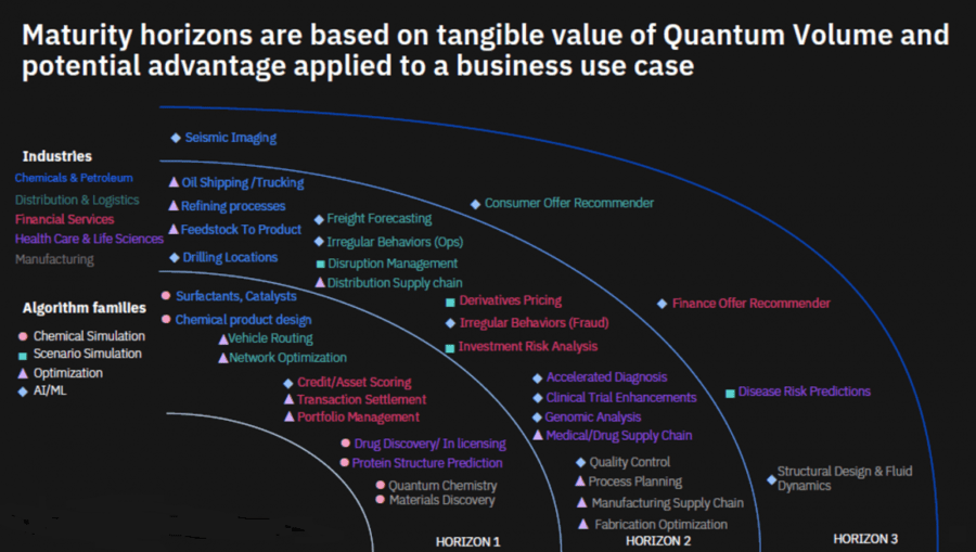
Now let me discuss potential quantum computing applications in detail:

1. Optimization:

Optimization problems exist in all industries and business functions and some of these problems take too long to be solved optimally with traditional computers. Two quantum approaches can be used to solve these problems:

-1. Quantum annealing is an optimization heuristic that is expected to surpass classical computers in certain optimization problems. Quantum annealing can be implemented on specialized quantum annealers which are far easier to build than a universal quantum computer. Currently such computers are available however, their supremacy over classical computers is yet to be decisively proven. Cheaper digital annealers simulate quantum annealers using classical computing and pose cost-effective alternatives.

-2. Universal quantum computers: They are capable of solving all types of computational problems. However, they will take longer to be commercially available as more research is required to increase their reliability

Companies such as JP Morgan, Airbus, Daimler are among the companies testing quantum systems for their optimization challenges

Some optimization problems from various industries where we need to rely on sub-optimal heuristics are listed below. Quantum computers can solve these problems and identify global optimum:

-1. Automotive:

-Optimizing large autonomous fleets

-2. Energy:

-Utilization prediction

-Grid optimization

-3. Finance:

-Automated trading (e.g. predicting financial markets)

-Risk analysis

-Portfolio optimization

-Fraud detection

-4. Insurance:

-Valuation of instruments, premiums in complex cases

-5. Logistics:

-Supply chain optimization

-Inventory optimization

-6. Manufacturing

-Design optimization (e.g. batteries, chips, vehicles etc.)

-7. Pharma:

-Drug interaction prediction

-Personalized medicine taking into account genomics

-8. Technology/software

-Machine learning

__

2. Research:

Quantum simulation can help scientist better understand molecule and sub-molecule level interactions which can lead to breakthroughs in chemistry, biology, healthcare and nanotechnology. Physical experiments and the analysis of the results are basic methods that used in chemistry research. Simulating these researches in the classical computer environment and accelerating the process without the need for physical experiments seems far away. On the other hand, noise, which appears to be a problem for quantum computers, can be useful in chemical research. The noise generated by simulations with quantum computations reveals properties about chemical reactions. For many applications of quantum devices, such as cryptography, this noise can be a tremendous limitation and lead to unacceptable levels of error. However, for chemistry simulations, the noise would be representative of the physical environment in which both the chemical system (e.g., a molecule) and the quantum device exist. This means that NISQ simulation of a molecule will be noisy, but this noise actually tells you something valuable about how the molecule is behaving in its natural environment. In this case, unlike other fields of application, it may not be necessary to wait for quantum computing to solve the noise problem for chemical and materials science applications. As a result, room temperature superconductors, long-life batteries and catalysts that do not require high temperature could be discovered. The molecular biology and healthcare also includes a process similar to chemical research, which can replace laboratory experiments with quantum computing simulations. Releasing a drug is a challenging process that takes many years and costs about $ 2.7 billion. By enabling investigations into the effects of diseases on the human body and simulations on molecular level, quantum computers can accelerate drug testing.

__

3. Cryptography:

Quantum computers have been proven to break the most common encryption algorithms such as the public key cryptographic system RSA. This problem can be solved by costly change of cryptography algorithms and as with all investments with uncertain rewards, it should be delayed as much as possible. However, delaying change of encryption techniques has an inherent risk, what if an actor builds quantum computer with sufficient power to break RSA and does not publish its findings? Since the investment necessary to break RSA with quantum encryption can only be afforded by mega corporations and governments, there is limited cause for concern for the average enterprise.

However, if you are communicating state-level secrets, you should probably be and you probably are making sure that your encryption is quantum-ready. There are already quantum-ready encryption algorithms that rely on problems other than integer factorization such as lattice based crypto systems or McEliece crypto system. Quantum cryptography is likely to provide quantum-ready encryption algorithms as well.

__

4. Industry specific applications:

There are numerous industry specific applications of quantum computing summarized in the figure below.

__

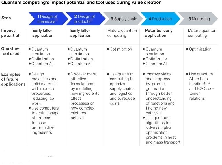
5. Navigation:

A GPS system cannot work everywhere on the planet, particularly underwater. A quantum computer requires atoms to be supercooled and suspended in a state that renders them particularly sensitive. In an effort to capitalize on this, competing teams of scientists are racing to develop a kind of quantum accelerometer that could yield very precise movement data. One promising effort to that end comes from France’s Laboratoire de Photonique Numérique et Nanosciences: An effort to build a hybrid component that pairs a quantum accelerometer with a classical one, then uses a high-pass filter to subtract the classical data from the quantum data. The result, if realized, would be an extremely precise quantum compass that would eliminate the bias and scale factor drifts commonly associated with gyroscopic components.

__

6. Seismology:

That same extreme sensitivity may also be exploited to detect the presence of oil and gas deposits, as well as potential seismic activity, in places where conventional sensors have to date been unable to explore; according to QuantIC, the quantum imaging technology hub led by the University of Glasgow. In July 2017, working with commercial photonics tools provider M Squared, QuantIC demonstrated how a quantum gravimeter detects the presence of deeply hidden objects by measuring disturbances in the gravitational field. If such a device becomes not only practical but portable, the team believes it could become invaluable in an early warning system for predicting seismic events and tsunamis.

___

7. Pharmaceuticals:

Classical computers are limited in terms of the size and complexity of molecules they can simulate and compare (an essential process in early drug development). If we have an input of size N, N being the number of atoms in the researched molecules, the number of possible interactions between these atoms is exponential (each atom can interact with all the others). Quantum computers will allow much larger molecules to be simulated. At the same time, researchers will be able to model and simulate interactions between drugs and all 20,000+ proteins encoded in the human genome, leading to greater advancements in pharmacology. Right from research into tackling diseases such as Alzheimer’s and multiple sclerosis, scientists have been utilizing software that models the behavior of artificial antibodies at the molecular level. Recently, neuroscience firm Biogen began partnering with IT consultancy Accenture and quantum computing research firm 1QBit to frame a new molecular simulation model in such a way that it can be executed on classical platforms, as well as present and future quantum platforms. One methodology developed by 1QBit’s researchers involves translating traditional molecular diagrams into graphs full of dots, lines, and curves that, while seemingly more confusing on the surface, map more directly to a quantum model of vectors and relationships.

__

8. Healthcare:

From a clinical healthcare perspective alone, the quantum computing technology could lead to “dramatic” accelerations in speed and performance. MRIs were basically invented because of our acquired understanding of quantum physics, and getting a true quantum computer will allow us to truly understand the nature of all matter, which means everything from better medicine with less side effects to better diagnostics. With increased computing available, clinicians could easily review CT scans over time and quickly identify changes and anomalies. Targeted chemotherapy protocols can be identified more quickly, and with more customization, with quantum computing’s enhanced data processing abilities. Targeted radiotherapy depends upon the ability to rapidly model and simulate complex scenarios to deliver the optimal treatment. Quantum computers would enable therapists to run more simulations in less time, helping to minimise radiation damage to healthy tissue. Quantum technologies could be used to provide faster, more accurate diagnostics with a variety of applications. Boosting AI capabilities will improve machine learning – something that is already being used to aid pattern recognition. High-resolution MRI machines will provide greater levels of detail and also aid clinicians with screening for diseases.

Potential solutions to COVID-19 can be found in the following areas using quantum computing:

1. the modelling and simulation of the spread of the virus,
2. the scheduling of nurses and other hospital resources,
3. assessing the rate of virus mutation,
4. the assessment of existing drugs as potential treatment,
5. speeding-up AI to rapidly suggest a vaccine,
6. quantum simulation can map the coronavirus’s proteins in hopes of revealing vulnerabilities that can be attacked with new drugs,
7. allocating patients to medical facilities as close as possible according to the patient’s symptoms, so as not to exceed the capacity of the medical facilities is challenging. This is a mathematical problem that can be done on a quantum-computing system that takes into account the distance from the origin of the patients to the medical facilities as well as the patient’s symptoms and the capacity of each medical facility.

Quantum computing isn’t yet far enough along that it could have helped curb the spread of Covid-19 outbreak. But this emerging field of computing will almost certainly help scientists and researchers confront future crises.

___

9. Finance:

-Automated, high-frequency trading

One potential application for quantum technologies is algorithmic trading – the use of complex algorithms to automatically trigger share dealings based on a wide variety of market variables. The advantages, especially for high-volume transactions, are significant.

-Fraud detection

Like diagnostics in healthcare, fraud detection is reliant upon pattern recognition. Quantum computers could deliver a significant improvement in machine learning capabilities; dramatically reducing the time taken to train a neural network and improving the detection rate.

___

10. Marketing

Quantum computers will have the ability to aggregate and analyse huge volumes of consumer data, from a wide variety of sources. Big data analytics will allow commerce and government to precisely target individual consumers, or voters, with communications tailored to their preferences; helping to influence consumer spending and the outcome of elections.

__

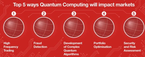
11. Weather Forecasting:

With so many variables to consider, accurate weather forecasts are difficult to produce. Machine learning using quantum computers will result in improved pattern recognition, making it easier to predict extreme weather events and potentially saving thousands of lives a year. Climatologists will also be able to generate and analyse more detailed climate models; proving greater insight into climate change and how we can mitigate its negative impact.

NOAA Chief Economist Rodney F. Weiher claims that nearly 30 percent of the US GDP ($6 trillion) is directly or indirectly affected by weather, impacting food production, transportation, and retail trade, among others. The ability to better predict the weather would have enormous benefit to many fields, not to mention more time to take cover from disasters.

While this has long been a goal of scientists, the equations governing such processes contain many, many variables, making classical simulation lengthy. As quantum researcher Seth Lloyd pointed out, “Using a classical computer to perform such analysis might take longer than it takes the actual weather to evolve!” This motivated Lloyd and colleagues at MIT to show that the equations governing the weather possess a hidden wave nature which are amenable to solution by a quantum computer.

Director of engineering at Google Hartmut Neven also noted that quantum computers could help build better climate models that could give us more insight into how humans are influencing the environment. These models are what we build our estimates of future warming on, and help us determine what steps need to be taken now to prevent disasters.

The United Kingdom’s national weather service Met Office has already begun investing in such innovation to meet the power and scalability demands they’ll be facing in the 2020-plus timeframe, and released a report on its own requirements for exascale computing.

__

12. Logistics:

Improved data analysis and modelling will enable a wide range of industries to optimise workflows associated with transport, logistics and supply-chain management. The calculation and recalculation of optimal routes could impact on applications as diverse as traffic management, fleet operations, air traffic control, freight and distribution.

_____

13. Energy usage:

Quantum computing could change the way the world uses energy:

Our connected devices are hiding a big secret. They use energy—a lot of it. Every time you use your phone, your computer, or your smart TV to access the internet, you’re sending data requests to warehouse-sized buildings around the world, full of hundreds of thousands of servers. These data centers are among the most energy-intensive systems on the planet, using approximately 10% of global electricity generation (though more conservative estimates put it at 3%).

Yet we’re still blindly making classic computers—and they’re getting bigger and even more energy dense. China is home to the most energy-intensive supercomputer in the world, the Tianhe-2 in Guangzhou. This machine uses about 18 megawatts of power, and is expected to be succeeded by the exascale Tianhe-3, which will only further increase this extraordinary level of energy consumption.

This is just one reason why quantum computing is key to the future. In addition to holding the potential to solve some of the world’s most computationally challenging problems, quantum computers use significantly less energy, which could lead to lower costs and decreased fossil-fuel dependency as adoption grows.

__

14. Exponentially Faster Data Analysis:

The explosion of the Internet, rapid advances in computing power, cloud computing, and our ability to store more data than was even considered possible only two decades ago has helped fuel the Big Data revolution of the 21st century, but the rate of data collection is growing faster than our ability to process and analyze it. In fact, 90 percent of all data produced in human history was produced within the last two years. As scientific instruments continue to advance and even more data is accumulated, researchers classical computing will be unable to process the growing backlog of data. Fortunately, scientists at MIT partnered with Google to mathematically demonstrated the ways in which quantum computers, when paired with supervised machine learning, could achieve exponential increases in the speed of data categorization. While only a theory now, once quantum computers scale sufficiently to process these data sets, this algorithm alone could process an unprecedented amount of data in record time.

__

15. Particle Physics:

Coming full circle, a final application of this exciting new physics might be… studying exciting new physics. Models of particle physics are often extraordinarily complex, confounding pen-and-paper solutions and requiring vast amounts of computing time for numerical simulation. This makes them ideal for quantum computation, and researchers have already been taking advantage of this. Researchers at the University of Innsbruck and the Institute for Quantum Optics and Quantum Information (IQOQI) recently used a programmable quantum system to perform such a simulation. Published in Nature, the team used a simple version of quantum computer in which ions performed logical operations, the basic steps in any computer calculation. This simulation showed excellent agreement compared to actual experiments of the physics described. “These two approaches complement one another perfectly,” says theoretical physicist Peter Zoller. “We cannot replace the experiments that are done with particle colliders. However, by developing quantum simulators, we may be able to understand these experiments better one day.”

_______

_______

Cloud-based quantum computing (quantum cloud computing):

Quantum computers truly do represent the next generation of computing. Unlike classic computers, they derive their computing power by harnessing the power of quantum physics. Because of the rather nebulous science behind it, a practical, working quantum computer still remains a flight of fancy. Give clients access to a quantum computer over the internet, and you have quantum cloud computing. Cloud-based quantum computing is the invocation of quantum emulators, simulators or processors through the cloud. Increasingly, cloud services are being looked on as the method for providing access to quantum processing. When users are allowed access to quantum computers through the internet it is known as quantum computing within the cloud.

IBM had connected a small quantum computer to the cloud and it allows for simple programs to be built and executed on the cloud. Many people from academic researchers and professors to schoolkids, have already built programs that run many different quantum algorithms using the program tools. Some consumers hoped to use the fast computing to model financial markets or to build more advanced AI systems. These use methods allow people outside a professional lab or institution to experience and learn more about such a phenomenal technology.

_

Cloud-based quantum computing is used in several contexts:

1. In teaching, teachers can use cloud-based quantum computing to help their students better understand quantum mechanics, as well as implement and test quantum algorithms.
2. In research, scientists can use cloud-based quantum resources to test quantum information theories, perform experiments, compare architectures, amongst other things.
3. In games, developers can use cloud-based quantum resources can create quantum games to introduce people to quantum concepts.

_

Existing platforms for Cloud-based quantum computing:

1. Forest by Rigetti Computing, which consists of a toolsuite for quantum computing. It includes a programming language, development tools and example algorithms.
2. LIQUi|> by Microsoft, which is a software architecture and toolsuite for quantum computing. It includes a programming language, example optimization and scheduling algorithms, and quantum simulators. Q#, a quantum programming language by Microsoft on the .NET Framework seen as a successor to LIQUi|>.
3. IBM Q Experience by IBM, providing access to quantum hardware as well as HPC simulators. These can be accessed programmatically using the Python-based Qiskit framework, or via graphical interface with the IBM Q Experience GUI. Both are based on the OpenQASM standard for representing quantum operations. There is also a tutorial and online community.

Currently available simulators and quantum devices are:

-Multiple transmon qubit processors. Those with 5 and 16 qubits are publicly accessible. Devices with 20 qubits are available through the IBM Q Network.

-A 32 qubit cloud-based simulator. Software for locally hosted simulators are also provided as part of Qiskit.

4. Quantum in the Cloud by The University of Bristol, which consists of a quantum simulator and a four qubit optical quantum system.
5. Quantum Playground by Google, which features a simulator with a simple interface, and a scripting language and 3D quantum state visualization.
6. Quantum in the Cloud by Tsinghua University. It is a four-qubit new quantum cloud experience based on nuclear magnetic resonance-NMRCloudQ.
7. Quantum Inspire by Qutech, providing access to QX, a quantum simulator backend. Three instances of the QX simulator are available, simulating up to 26 qubits on a commodity cloud-based server and up to 37 qubits using 16 ‘fat’ nodes on Cartesius, the Dutch national supercomputer of SurfSara. Circuit based quantum algorithms can be created through a graphical user interface or through the Python-based Quantum Inspire SDK, providing a backend for the projectQ framework, the Qiskit framework. Quantum Inspire provides a knowledge base with user guides and some example algorithms written in cQASM.
8. Forge by QC Ware, providing access to D-Wave hardware as well as Google and IBM simulators. The platform offers a 30-day free trial including one minute of quantum computing time.

_

Quantum computing as a service (QCaaS):

As with any new technological innovation, there is a risk that the hype outpaces product development, which could negatively impact perceptions and investments. In the case of quantum computing, this is called quantum winter. Hype in the media is creating awareness and advancement, but also setting unrealistic expectations for timing and capabilities. This level of hype inevitably leads to disillusionment, which is dangerous, as quantum computing requires sustained, focused investment for the long term. The hype around quantum computing makes it interesting as an investment. However, the fundamental physics are still in development, and consistent results won’t appear for at least 5 to 10 years — and possibly much longer. Therefore, any investments made in pursuit of quantum computing opportunities must pay off in monetizable discoveries.

Logistically, quantum computers are difficult to maintain and require specialized environments cooled to 0.015 Kelvin. The quantum processor must be placed in a dilution refrigerator shielded to 50,000 times less than the earth’s magnetic field and placed in a high vacuum to 10 billion times lower than atmospheric pressure. It will also need calibration several times per day. For most organizations, this is not feasible. Gartner recommends that organizations interested in quantum computing leverage quantum computing as a service (QCaaS) to minimize risk and contain costs. By 2023, 95% of organizations researching quantum computing strategies will utilize QCaaS.

_

Amazon Web Services (AWS) launches Braket, a quantum computing as a service:

E-commerce giant, Amazon has silently placed its cards on the table. Understanding the potential to solve computational problems that are beyond the reach of classical computers by harnessing the laws of quantum mechanics to build more powerful tools for processing information, the cloud computing platform of this e-comm giant joined hands with D-Wave, IonQ and Rigetti and unveiled its all-new quantum computing service known as Braket. Recently AWS officially announced the preview launch of Braket, its first-ever quantum computing service. The term Braket is derived from “bra–ket notation” which is a common notation for quantum states in quantum mechanics. Amazon’s Braket is a fully managed service that helps to get started with quantum computing by providing a development environment to explore and design quantum algorithms, test them on simulated quantum computers, and run them on the choice of different quantum hardware technologies.

How Braket Helps:

Gaining access to quantum computing hardware to run the algorithms and optimize designs can be expensive and inconvenient. Also, programming quantum computers to solve a problem requires a new set of skills. Amazon Braket helps in overcoming these difficulties by providing a service that lets developers, researchers, and scientists explore, evaluate, and experiment with quantum computing.

This service allows users to choose from a variety of quantum computers which include gate based superconductor computers from Rigetti, quantum annealing superconductor computers from D-Wave, and ion trap computers from IonQ. Braket also allows users to design their own quantum algorithms from scratch or to choose from a set of pre-built algorithms. Once the algorithm gets defined, Amazon Braket provides a fully managed simulation service to help in troubleshooting and verifying the implementation. A user can then run the algorithm on any of the above-mentioned quantum computers.

Furthermore, in order to make it easier for the users to develop a hybrid algorithm which is a combination of both classical and quantum tasks, Amazon Braket helps in managing classical compute resources and establish low-latency connections to the quantum hardware.

______

______

Quantum computing vs. classical (conventional or traditional) computing:

_

As the reality of a quantum computer comes closer, it is useful for us to understand both how one functions and how it’s different from a traditional (classical) computer.

The first thing to bear in mind is that they use different basic units of data: ‘bits’ and ‘qubits’. Every element of a classical computer is written in binary code (1s and 0s) and is translated into electricity: high voltage is represented by 1, and low voltage by 0. In quantum computing, qubits are the basic unit and their value can be 1, 0, or 1 and 0 simultaneously, overlapping (superposition) and intertwining (entanglement) according to the laws of physics. This means that qubits, as opposed to bits, can take on various values at one time and can perform calculations that a conventional computer cannot.

In classical computing we know how to solve problems thanks to computer language (AND, OR, NOT) used when programming. Operations that are not feasible in bit computing can be performed with a quantum computer. In a quantum computer all the numbers and possibilities that can be created with N qubits are superimposed (if there are 3 qubits, there will be 8 simultaneous possible permutations.) With 1,000 qubits the exponential possibilities far exceed those that we have in classical computing.

Currently, in contrast to classical computing, there are no quantum computing languages per se. A quantum computer isn’t suitable for performing day-to-day tasks. They don’t have memory or a processor. We only have a group of qubits that we use to write information, and we work with those. There isn’t an architecture as complicated as the architecture for a conventional computer. Today, quantum machines are primitive systems akin to a calculator at the turn of the last century, but their computing power for very specific problems is much greater than a traditional computer’s. There is a dichotomy between what appears very simple and what it does, which is very powerful.

Traditional software development, using classical computers, translates a high-level programming language (for example, Java) to operations performed on a large number of (hardware) transistors. The flow of this process is as follows: Java source code is compiled into platform-independent bytecode, which is translated to platform-specific machine code. This allows Java code to work on different operating systems and architectures. The machine code leverages a number of basic operations (gates) acting on memory. The main hardware component to achieve this is the well-known transistor. Performance improvements from the past decades have mainly been driven by advantages in hardware technology. The size of a single transistor has been reduced drastically, and more transistors per square millimeter allow for more memory or more processing power.

All information is processed and understood by a computer using this binary language composed of bits (0 or 1). When you break a computer down, you will find a bunch of silicon chips with circuits of logic gates made up of transistors or switches which function using voltage. A high voltage represents on state of the switch equivalent to 1 and a low equivalent to 0. All forms of data be it text, music, audio, video or software are ultimately encoded and stored by the computer as binary in the computer’s memory.

Quantum computing is disruptive, because it doesn’t use a classical transistor as the basic building block; it uses qubits. Not only are the basic building blocks different, the gates are different as well. Hence, the flow of process discussed before does not apply to quantum computing. However there is a growing consensus among scientists that quantum computers are particularly good for some problems, while classical computers are best for other problems.

_

Difference between conventional (classical) computing and quantum computing:

Conventional Computing	Quantum Computing
Conventional computing is based on the classical phenomenon of electrical circuits being in a single state at a given time, either on or off.	Quantum computing is based on the phenomenon of Quantum Mechanics, such as superposition and entanglement, the phenomenon where it is possible to be in more than one state at a time.
Information storage and manipulation is based on “bit”, which is based on voltage or charge; low is 0 and high is 1.	Information storage and manipulation is based on Quantum Bit or “qubit”, which is based on the spin of electron or polarization of a single photon.
The circuit behavior is governed by classical physics.	The circuit behavior is governed by quantum physics or quantum mechanics.
Conventional computing use binary codes i.e. bits 0 or 1 to represent information.	Quantum computing use Qubits i.e. 0, 1 and superposition state of both 0 and 1 to represent information.
CMOS transistors are the basic building blocks of conventional computers.	Superconducting Quantum Interference Device or SQUID or Quantum Transistors are the basic building blocks of quantum computers.
In conventional computers, data processing is done in Central Processing Unit or CPU, which consists of Arithmetic and Logic Unit (ALU), processor registers and a control unit.	In quantum computers, data processing is done in Quantum Processing Unit or QPU, which consists of a number of interconnected qubits.

_

The conventional computer’s Achilles heel:

The fact is that a computational task such as quickly finding the prime factors for very large integers is probably out of reach for even the fastest conventional computers of the future. The reason behind this is that finding the prime factors of a number is a function that has exponential growth. What’s exponential growth? Some things grow at a consistent rate and somethings grow faster as the number of “things” you have also grows. When growth becomes more rapid (not constant) in relation to the growing total number, then it is exponential. Exponential growth is extremely powerful. One of the most important features of exponential growth is that, while it starts off slowly, it can result in enormous quantities fairly quickly — often in a way that is shocking.

Let’s move on to real world exponential problem.

Prime Factorization.

Take the number 51. See how long it takes you to find the two unique prime numbers that you can multiply together to generate it. If you’re familiar with these kinds of problems, it probably only took you a few seconds to find that 3 and 17, both primes, generate 51. As it turns out, this seemingly simple process, lies at the heart of the digital economy and is the basis for our most secure types of encryption. The reason we use this technique in encryption is because as the numbers used in prime factorization get larger and larger, it becomes increasingly difficult for conventional computers to factor them. Once you reach a certain number of digits, you find that it would take even the fastest conventional computer months, years, centuries, millennia, or even countless eons to factor it.

Other equally stubborn problems at the heart of modern science and mathematics include certain molecular modeling and mathematical optimization problems which promise to crash any supercomputer that dares to come anywhere near them.

_

Enter the quantum computer:

Conventional computers are strictly digital, and rely purely on classical computing principles and properties. Quantum computers, on the other hand, are strictly quantum. Accordingly, they rely on quantum principles and properties — most importantly superposition and entanglement — that make all the difference in their almost miraculous capacity to solve seemingly insurmountable problems.

Superposition:

The key features of an ordinary computer—bits, registers, logic gates, algorithms, and so on—have analogous features in a quantum computer. Instead of bits, a quantum computer has quantum bits or qubits, which work in a particularly intriguing way. Where a bit can store either a zero or a 1, a qubit can store a zero, a one, both zero and one, or an infinite number of values in between—and be in multiple states (store multiple values) at the same time! A gentler way to think of the numbers qubits store is through the physics concept of superposition (where two waves add to make a third one that contains both of the originals). If you blow on something like a flute, the pipe fills up with a standing wave: a wave made up of a fundamental frequency (the basic note you’re playing) and lots of overtones or harmonics (higher-frequency multiples of the fundamental). The wave inside the pipe contains all these waves simultaneously: they’re added together to make a combined wave that includes them all. Qubits use superposition to represent multiple states (multiple numeric values) simultaneously in a similar way.

Just as a quantum computer can store multiple numbers at once, so it can process them simultaneously. Instead of working in serial (doing a series of things one at a time in a sequence), it can work in parallel (doing multiple things at the same time). Only when you try to find out what state it’s actually in at any given moment (by measuring it, in other words) does it “collapse” into one of its possible states—and that gives you the answer to your problem in probability. Estimates suggest a quantum computer’s ability to work in parallel would make it millions of times faster than any conventional computer… if only we could build it!

If you want to understand what gives rise to superposition then you are going to first need to understand the idea of Wave/Particle Duality.

Entanglement:

It is known that once two quantum systems interact with one another, they become hopelessly entangled partners. From then on, the state of one system will give you precise information about the state of the other system, no matter how far the two are from one another. Seriously, the two systems can be light years apart and still give you precise and instantaneous information about each other.

Suppose you have two electrons, A and B. Once you have them interact in just the right way, their spins will automatically get entangled. From then on, if A’s spin is Up, B’s spin will be Down, like two kids on a seesaw, except that this holds true even you take A and B to opposite ends of the Earth (or the galaxy, for that matter). Despite the thousands of miles (or light years) between them, it’s been proven that if you measure A to have spin Up, you will know instantly that B’s spin is Down. But wait: we’ve already learned that these systems don’t have precise values for states such as spin, but rather exist in a murky superposition, prior to measurement. So does our measuring A actually cause B to instantaneously collapse to the opposite value, even when the two are light years apart? If so, then we have yet another problem on our hands, because nothing between two systems can travel faster than the speed of light. So what gives this? All told, we honestly don’t know. All we know is that quantum entanglement is real, and that you can leverage it to work wonders.

_

The quantum system uses qubits as the smallest discrete units to represent information, which may be electrons with spins, photons with polarization, trapped ions, semiconducting circuits etc. The property of quantum mechanics comes into play as a single qubit can exist not only, in two discrete energy states, low and high (similar to 0 and 1) but it can also exist in a superposition state where in it exists in both states at once. When measured however, the superposition fades and one of the two distinct states is returned based on the probabilities of each state.

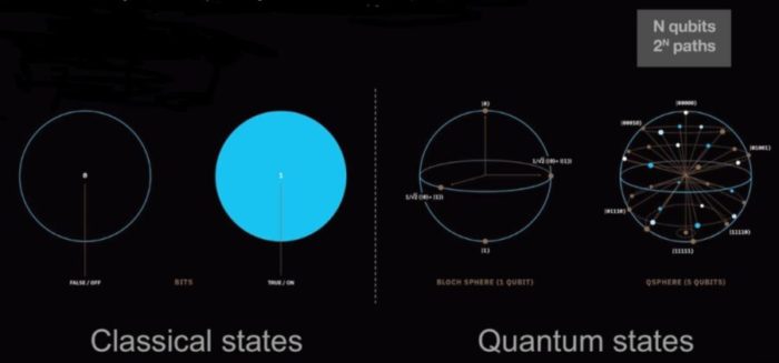
When using two qubits instead of a single qubit 4 discrete energy states exist, (2 discrete states for each qubit) and a qubit can even exist in a superposition of these states. Similarly using n qubits, 2ⁿ states are achieved which exist as combinations of 0s and 1s in parallel.

So this gives a way to represent information. The next step is to process information, which requires manipulation of these qubits. This is brought about by the use of special quantum logic gates and quantum algorithms such as Shor’s algorithm and Grover’s algorithm which function using the principles of quantum mechanics of superposition, entanglement and measurement. Without going into the complicated details of the quantum phenomena, the state of the qubits is manipulated by application of precise electromagnetic waves, microwaves and amplification functions as defined by the algorithms.

Just as conventional computers are built bit by bit with transistors that are either On or Off, quantum computers are built qubit by qubit with electrons in spin-states that are either Up or Down (once measured, of course). And just as transistors in On/Off states are strung together to form the logic gates that perform classical computations in digital computers, electrons in Up/Down spin-states are strung together to form the quantum gates that perform quantum calculations in quantum computers. Yet stringing together individual electrons (while preserving their spin states) is far, far easier said than done.

___

Traditional computers utilize the flow of electricity and can be turned on or off at switches inside circuits. Whether a switch is on or off generates the ones and zeros that underlie all computer code. This is what Alan Turing discovered in his pioneering work: Simple rules for turning those switches on and off can be used to solve any mathematical problem. These zeros and ones are called bits, and they are the smallest bit of information a computer stores.

Quantum computers, on the other hand, are not built upon using the flow of electricity. They rely instead on the physical properties of electrons, photons, and other tiny bits of matter that are subject to the laws of quantum mechanics. These bits of matter can do a lot more than just be turned on and off. Actually, on and off aren’t really words that make sense in quantum physics. This kind of tiny matter is best described in states called amplitudes (like waves, since the tiniest bits of matter can act as both particles and waves). A particle can have two different amplitudes at the same time — a state called superposition. They can also be entangled, meaning a change in one particle instantly changes another. The amplitudes of particles can also cancel one another out like opposing waves in water would. Also, the smallest particles in nature don’t really exist in a point in space but they exist as a probability of existing.

Quantum mechanics are the rules that make reality. Take an electron. According to classical physics (think Newton’s laws of motion), electrons should spiral into the center of atoms, rendering them useless. What quantum mechanics ultimately says is there are all these pathways where the electron can spiral into the nucleus, but they all cancel each other out. It’s like the electron itself is a computer, sorting through all the possible paths it can take before finding the right ones. In a sense, the electron has solved the problem of its own existence.

Amazingly, what quantum computer engineers are doing is tapping into the chaotic logic of the quantum world to solve problems. Like a normal computer with its switches to control the flow of electricity, they build hardware to influence quantum states. (A part of the research into quantum computing is figuring out what the optimal hardware should be.) They’re trying to choreograph quantum interactions in a way so the wrong answers to big problems get cancelled out.

In a normal computer, a bit can be in two states — on or off. Zero or one. But a qubit — a.k.a. a quantum bit — can be in many states at once. That means a single qubit can contain exponentially more information than a normal bit. That’s a bit like having four regular computers running side by side. If you add more bits to a regular computer, it can still only deal with one state at a time. But as you add qubits, the power of your quantum computer grows exponentially.

What it boils down to is that a quantum computer can crunch through some enormous problems really quickly. For instance, a lot of cybersecurity depends on computers multiplying huge prime numbers. It’s really really hard for traditional computers to reverse this process, to find the prime numbers that resulted in the bigger number and crack the encryption. But quantum computers could. In a quantum computing world, we may need even stronger security protections, perhaps even those derived from quantum mechanics itself.

Scientists hope quantum computers may lead to better, quicker ways to solve optimization problems. When you have many different choices in front of you, how do you choose the ideal path? These types of questions strain traditional computers but could, potentially, be a breeze for quantum computers, which could sort through all the possible parts at once. A traditional computer has to try out each path one at a time. Though, we’re not going to be able to run applications like that for a while because the quantum hardware just isn’t advanced enough.

Quantum computers are hard to build, are prone to generating errors, and their components are often unstable. Right now, what Google has shown is a proof of concept: that quantum computers can solve problems in a way traditional computer can’t. Its machine runs 54 qubits. But this is a tiny fraction of the one million qubits that could be needed for a general-purpose machine.

Quantum computers don’t really do anything practical yet. The test problem Google ran for their paper was — and this is a simplification — to see if a random number generator was truly random. They’re validating that their hardware is doing what they think it’s supposed to be doing, checking that with the quantum computer they can perform the computation with many fewer steps and much faster than a classical computer.

Perhaps most of the more immediate uses would just be to use quantum computers to simulate the frenzied world of quantum mechanics and better understand it.

We can use a quantum computer as a general simulator of nature on the microscopic scale and use it to predict what a protein will do, help design a drug that will bind to a receptor in the right way, and help design new chemical reactions … design better batteries. You would only need one or two successes to make this whole thing worthwhile.

____

Two key factors make quantum computers a billion times more powerful than the most powerful supercomputer known to us today. These are:

1. Parallelism
2. Exponential increase in computing ability with the addition of each qubit

This gives quantum computers processing power that is beyond the scope of a classical computer.

One example:

Four classical Bits can be transformed in 2⁴ combinations i.e. 16 combinations as follows-

0000    0001    0010    0011

0100    0101    0110    0111

1000    1001    1010    1011

1100    1101    1110    1111

That’s 16 possible combinations, out of which we can use only one at a time. Our CPU calculates at average 2.4GHz, apparently, it looks like that all combinations are calculated simultaneously but of course they are distinct from each other and CPU calculate one at a time each combination. Although simultaneous calculation can be done by having more than 1 CPU in the machine and that’s is called as Multiprocessing but that’s a different thing. The fact is that our CPU calculates each combination one at a time. Here arises a big and advanced research question – can all of them be used simultaneously at once without having any multiprocessors?

Yes, in quantum computing.

4 qubits can process 16 combinations simultaneously at once.

____

Quantum computers have four fundamental capabilities that differentiate them from today’s classical computers: (1) quantum simulation, in which quantum computers model complex molecules; (2) optimization (that is, solving multivariable problems with unprecedented speed); (3) quantum artificial intelligence, with better algorithms that could transform machine learning across industries as diverse as pharma and automotive; and (4) prime factorization, which could revolutionize encryption.

____

Software developers for classical computers can rely on integer and floating point numbers, algebraic expressions with arithmetic operators and trigonometric functions, conditional branching, looping, and nested functions — but none of these constructs even exists in a quantum computer.

To put it most simply, a classical computer provides a rich computation model, closely matching human conceptions of mathematics and logic, while with a quantum computer you’re relying only on the raw physics of quantum mechanics, with none of the rich abstractions and semantics that classical computing provides.

Quantum computing revolves around the qubit and its quantum states, which can be superimposed and entangled with another qubit, while much of classical computing revolves around numbers, integer and decimal, and text. There is more than a little mismatch between these two worlds.

Classical computing has always been a bit too deterministic compared to the uncertainty, ambiguity, and confusion that surrounds most human endeavours. But the point remains that real people and software developers can more easily relate to the determinism of classical computers than to the uncertain probabilistic nature of quantum computing. Classical computing revolves around the abstract concept of a Turing machine, whose semantics are not rooted in either physics or quantum mechanics. A Turing machine represents computable functions, in a traditional mathematical sense. At present, there is no such abstraction on any current or even proposed quantum computer. Again, the software developer is forced to think and operate on the level of the raw physics, with no simplifying abstractions to relate to normal mathematics and logic, like evaluating algebraic expressions, calling functions, or conditionally executing operations.

A critical issue for algorithms and hardware is scalability. It is easy to demonstrate a solution to a problem on a relatively small scale, but that leaves open the question of how that solution scales to a much larger amount of data and processing power. Quantum computing does have the prospect of scaling better than classical computing, but realizing that potential is another matter. Limited connectivity of qubits in current quantum computers has an impact on scalability. And that says nothing about whether or how any particular algorithm scales. We have a lot of tricks and techniques for scaling algorithms on classical computers, but very little of that is relevant to current quantum computers. The point here is not that quantum computing is impossible for mere mortals to relate, but simply that we have a great distance to travel before we arrive at a state of affairs where moderately skilled software developers can swiftly proceed through complex quantum computing tasks.

In short, we need a far richer algorithmic infrastructure — and hardware which supports it — before we can tackle more than just a few, high-value niche applications.

_____

_____

The advantages and disadvantages of Quantum Computing:

The advantages of Quantum Computing:

It has been shown in theory that a quantum computer will be able to perform any task that a classical computer can, and recent IBM show case demonstrated it as well. However, this does not necessarily mean that a quantum computer will outperform a classical computer for all types of task (in particularly once you add in the cost in the consideration). If we use our classical algorithms on a quantum computer, it will simply perform the calculation in a similar manner to a classical computer. In order for a quantum computer to show its superiority it needs to use new what we call ‘quantum algorithms’ which can exploit the phenomenon of quantum parallelism. In another word, if just repeat the same algorithms, nothing much to be gain.

Such algorithms are not easy to formulate, it take time and research and development (R&D) effort and resources to discover what work. A well know example for one of the algorithm is the quantum factorization algorithm created by Peter Shor of AT&T Bell laboratories. What the algorithm do is tackles the problem of factorizing large numbers into its prime factors. And this task is classically very difficult to solve (based on current technology). Shor’s algorithm cleverly uses the effects of quantum parallelism to give the results of the prime factorization problem in a matter of seconds whereas a classical computer would take, in some cases, more than the age of the universe to produce a result!

The disadvantages of Quantum Computing:

First thing first, it is the cost. Today, a single qubit will set you back $10,000 – and that’s before you consider research and development costs. At that price, a useful universal quantum computer – hardware alone – comes in at least $10bn. This for a machine whose true commercial value is far from guaranteed. To make quantum computers commercially viable, the cost per qubit will have to drop dramatically. But how this will happen, no one knows. D-Wave is now shipping its new $15 million, 10-foot tall quantum computer called the D-Wave 2000Q with 2000 qubits but their hardware is based on an ‘adiabatic’ process called ‘quantum annealing’ that other pioneers have dismissed as ‘restrictive’ and ‘a dead end’.

The biggest disadvantage of quantum computing (QC), is that it works for only very short periods of time, times that are too short to solve any problems. By depending on entanglement, then that phenomenon has to work with a very high expectancy of being dependable or be able to do the action of entanglement or combining two or more states at the same time for sufficiently long times to achieve useful operational times of a QC. If that action of combining multiple states does not do what it predicts in a dependable way, then quantum computing will not work as well as otherwise expected, or if it does work dependably, will work dependably by being forced to do so. What that means is that the less dependably that entanglement works, the more additions have to be made to the system, to make or force entanglement to seem to work dependably. This leads to an iterative build up of the components or configurations of components, so as to achieve the level of dependability that is required. That achievement of getting entanglement, to work over sufficiently long periods of time to allow QC, in turn to work, is what is currently the bottle neck that is slowing down the development of quantum computing.

At the initial stage of QC theory, there seemed to be the promise of making entanglement to be sufficiently stable to make QC a sure thing. Recently, the stability of entangled bits has become an issue. This issue has developed to the point, that the qubits that depend on entanglement to work, are so unstable, as to require trying various new ways of achieving entanglement. The initial method consisted of producing a pair of electrons with complementary properties. Each newer method has added more components to the point where the final system achieved has become even more unstable and/or cumbersome to do anything.

______

______

Quantum computing hype:

It makes sense that sci-fi-level myths might surround a technology that must be stored in a container colder than interstellar space and has the potential to solve some of the world’s most challenging problems. CIOs have been inundated with quantum computing hype: “Quantum computers will operate faster than the speed of light,” or “Quantum computers will replace conventional systems” or “Quantum computing will render all security encryption algorithms obsolete.”

The truth is that quantum solutions could revolutionize the entire IT industry with major economic, industrial, academic and societal impacts. But they won’t operate faster than light travels or replace current computing systems, and although they’ll challenge some security encryptions, they won’t render them all obsolete overnight.

Quantum computing is heavily hyped and evolving at different rates, but it should not be ignored. It holds great promise, especially in the areas of chemistry, optimization, machine learning and AI to name a few. Today’s data scientists simply cannot address key opportunities in these areas because of the compute limitations of classic computer architectures.  A recent report by the National Academies of Sciences, Engineering, and Medicine throws some cold water on the hype smoldering around quantum computing. The report finds no commercially viable applications for near-term quantum computers that cannot already be tackled with conventional computers. This National Academies report concludes that early quantum computers may not beat out conventional computers in chemistry simulations or other applications. Qubits are sensitive devices, and prone to error. To get the right answer from a quantum computer, researchers either have to repeat a calculation an unreasonable number of times, or build a quantum computer with millions of qubits. And the challenge in scaling up is not in the fabrication—after all, the semiconductor industry can pack billions of devices in small areas—but in the operation. Even tens of qubits nestled together in one array start interfering with one another, causing errors. This error correction problem, along with other issues, led the report’s committee to conclude that “there is no publicly known application of commercial interest based upon quantum algorithms that could be run on a near-term analog or digital NISQ computer that would provide an advantage over classical approaches.”

_

Quantum computers, specifically the code needed to run them, are not ready yet. The most over-hyped aspect of quantum computing is the possible near-term algorithms because we do not know which if any will work on devices within the next three to five years, and which can be run efficiently on current digital computers. This paucity of appropriate code, much of which must be developed from the ground up, is just one hurdle that quantum computers must overcome before they are ready for widespread commercial use.

Google’s recent 53-qubit demonstration [of quantum computing] is akin to the Wright brothers’ first flights at Kitty Hawk. Their plane, the Wright Flyer, was not the first to fly. It didn’t solve any pressing transportation problem. Nor did it herald widespread adoption — commercial aviation would only gradually emerge over the next few decades. What the Wright Flyer did and what the quantum computers are doing now are simply proofs of concept. Quantum computers are nascent. To realize their promise, we will need to build robust, reproducible machines and develop the algorithms to use them. Engineering and technology development take time.

_

It is not helpful when the media makes wild, speculative claims. And it’s equally unhelpful when managers, executives, and promoters help to fuel those wild, speculative efforts. The only real solution is to patiently await real progress on both actual hardware and production-quality algorithms and code. And of course, we need to do more to accelerate progress on both fronts. Meanwhile, we should be doing more the pump the breaks on the unprecedented levels of hype and folklore.

Some examples of past and current wild claims:

1. Quantum computers break current encryption schemes. Not even close.
2. Shor’s algorithm is able to factor large prime numbers — to crack encryption schemes. Not even close. Researchers are still struggling with integer factorization schemes. The reality is that to break today’s encryption requires a large-scale and fault tolerant quantum computer, and we aren’t there yet. Therefore, we’re unlikely to see a quantum computing-driven security breach in the near future.
3. Grover’s algorithm can search databases. No, not really. Most databases are a lot more complex than simple, linear bit strings.

_

Will Quantum Computers replace Traditional Computing?

No.

Traditional computers don’t become obsolete when quantum computers finally reach commercial viability. It is important to understand that quantum computers will not replace classical computers. Quantum computers’ fundamental properties complement the traditional systems. It is fundamental to understand that quantum computers only fare better than classic systems when it comes to solve a very particularly category or class of problems (non-polynomial or NP), in other cases, their classic counterpart will perform as well or even better. That’s because the strength of quantum computers, having intermediate states somewhere between yes and no, can help the enterprise solve some forms of intractable classical problems that “blow up” or become extremely time-consuming with traditional computers, but they are not efficient for many of today’s other computing processes. The 0s and 1s of today’s computers are just fine for many computing applications, and there’s no need to completely replace traditional computers with quantum computers even if that were feasible.

Quantum computers therefore most likely will be a subset of the full computing landscape, just like there are processors built for graphics or AI but also other types of processors in use.

This means that a generation of computer science students also will need to learn how to use and code quantum computers for the coming emergence of the technology. From computer science courses to chemistry and business classes, students should be getting ‘quantum ready’.

Quantum computing is real, and it will have an impact on the world. But we’re not there yet, and everything isn’t going to change once quantum computers do reach the point of commercial viability. The emergence of quantum computers is more like the slow emergence of commercial aviation. The rise of flight did not mark the ‘beginning of the end’ for other modes of transportation — 90 percent of commercial shipping is still done today by ships.

_

Classical applications are poor fits for quantum systems:

Typical office work is not going to be improved by quantum computers; this is not a technology that an average accountant can utilize to improve their work. Quantum computers are not very good at the three Rs–reading, writing and arithmetic. They don’t like to read big databases, they can’t give you very big complicated readouts, and they don’t do regular arithmetic as well as a regular old classical computer.

The difficulty of attempting classic calculations on quantum computers is not widely understood, leading to optimistic predictions about their applicability for general-purpose use cases.

Suppose that you have a 200-layer deep neural network, 50 nodes per layer. That’s 200 by 50 by 50 weights that you need after you’re done training… let’s pretend that each of those weights as 50 bits, setting up an example of processing a petabyte of data using a machine learning algorithm. In in principle we could store [one petabyte] in 50 qubits. However, those have to be 50 perfect qubits. The current generation of quantum computers–Noisy Intermediate-Scale Quantum (NISQ) systems–use imperfect qubits which are subject to environmental noise, and are operable for a short time before reaching decoherence. It is possible for a quantum computer to combine noisy qubits to simulate a perfect qubit, with conversion around 1,000 noisy qubits for 1 good qubit. However, the big problem is that no one has any idea how to efficiently take that petabit of information and encode it in 50 cubits. There is no algorithm for that. There’s no such thing as a quantum hard drive. Every time the neural network is run, the data set must be re-loaded–which is not yet possible, and poses a large encumbrance for adoption of quantum computers. You can only get one classical bit of information out of every qubit. You have to re-run this 200 by 50 by 50 many times, and then carefully plan measurements so that each time you extract a unique weight. Each time you are doing that run, you re-encoding that petabit of data into the quantum register.

______

______

Quantum Computing scepticism:

Several Objections:

1. Works on paper, not in practice.
2. Violates Extended Church-Turing Thesis.
3. Not enough “real physics.”
4. Small amplitudes are unphysical.
5. Exponentially large states are unphysical.
6. Quantum computers are just souped-up analog computers.
7. Decoherence will always be worse than the fault-tolerance threshold.
8. Errors aren’t independent.

________

Will useful quantum computer be constructed in the foreseeable future?

The basic idea of quantum computing is to store and process information in a way that is very different from what is done in conventional computers, which are based on classical physics. Boiling down the many details, it’s fair to say that conventional computers operate by manipulating a large number of tiny transistors working essentially as on-off switches, which change state between cycles of the computer’s clock. The state of the classical computer at the start of any given clock cycle can therefore be described by a long sequence of bits corresponding physically to the states of individual transistors. With N transistors, there are 2^N possible states for the computer to be in. Computation on such a machine fundamentally consists of switching some of its transistors between their “on” and “off” states, according to a prescribed program.

In quantum computing, the classical two-state circuit element (the transistor) is replaced by a quantum element called a quantum bit, or qubit. Like the conventional bit, it also has two basic states. Although a variety of physical objects could reasonably serve as quantum bits, the simplest thing to use is the electron’s internal angular momentum, or spin, which has the peculiar quantum property of having only two possible projections on any coordinate axis: +1/2 or –1/2 (in units of the Planck constant). For whatever the chosen axis, you can denote the two basic quantum states of the electron’s spin as ↑ and ↓.

Here’s where things get weird. With the quantum bit, those two states aren’t the only ones possible. That’s because the spin state of an electron is described by a quantum-mechanical wave function. And that function involves two complex numbers, α and β (called quantum amplitudes), which, being complex numbers, have real parts and imaginary parts. Those complex numbers, α and β, each have a certain magnitude, and according to the rules of quantum mechanics, their squared magnitudes must add up to 1. That’s because those two squared magnitudes correspond to the probabilities for the spin of the electron to be in the basic states ↑ and ↓ when you measure it. And because those are the only outcomes possible, the two associated probabilities must add up to 1. For example, if the probability of finding the electron in the ↑ state is 0.6 (60 percent), then the probability of finding it in the ↓ state must be 0.4 (40 percent)—nothing else would make sense.

In contrast to a classical bit, which can only be in one of its two basic states, a qubit can be in any of a continuum of possible states, as defined by the values of the quantum amplitudes α and β. This property is often described by the rather mystical and intimidating statement that a qubit can exist simultaneously in both of its ↑ and ↓ states.

In a system with two qubits, there are 2² or 4 basic states, which can be written (↑↑), (↑↓), (↓↑), and (↓↓). Naturally enough, the two qubits can be described by a quantum-mechanical wave function that involves four complex numbers. In the general case of N qubits, the state of the system is described by 2^N complex numbers, which are restricted by the condition that their squared magnitudes must all add up to 1.

While a conventional computer with N bits at any given moment must be in one of its 2^N possible states, the state of a quantum computer with N qubits is described by the values of the 2^N quantum amplitudes, which are continuous parameters (ones that can take on any value, not just a 0 or a 1). So a quantum computer with N qubits would be in 2^N states simultaneously. This is the origin of the supposed power of the quantum computer, but it is also the reason for its great fragility and vulnerability.

How is information processed in such a machine? That’s done by applying certain kinds of transformations—dubbed “quantum gates”—that change these parameters in a precise and controlled manner.

Experts estimate that the number of qubits needed for a useful quantum computer, one that could compete with your laptop in solving certain kinds of interesting problems, is between 1,000 and 100,000. So the number of continuous parameters describing the state of such a useful quantum computer at any given moment must be at least 2^1,000.  That’s a very big number indeed. How big? It is much, much greater than the number of subatomic particles in the observable universe.

In other words, useful quantum computer needs to process a set of continuous parameters that is larger than the number of subatomic particles in the observable universe.

Now, in any real-world computer, you have to consider the effects of errors. In a conventional computer, those arise when one or more transistors are switched off when they are supposed to be switched on, or vice versa. This unwanted occurrence can be dealt with using relatively simple error-correction methods, which make use of some level of redundancy built into the hardware.

In contrast, it’s absolutely unimaginable how to keep errors under control for the 2^1,000 continuous parameters that must be processed by a useful quantum computer. Yet quantum-computing theorists have succeeded in convincing the general public that this is feasible. Indeed, they claim that something called the threshold theorem proves it can be done. They point out that once the error per qubit per quantum gate is below a certain value, indefinitely long quantum computation becomes possible, at a cost of substantially increasing the number of qubits needed. With those extra qubits, they argue, you can handle errors by forming logical qubits using multiple physical qubits.

How many physical qubits would be required for each logical qubit? No one really knows, but estimates typically range from about 1,000 to 100,000. So the upshot is that a useful quantum computer now needs a million or more qubits. And the number of continuous parameters defining the state of this hypothetical quantum-computing machine—which was already more than astronomical with 1,000 qubits—now becomes even beyond human imagination.

In light of all this, it’s natural to wonder: When will useful quantum computers be constructed? The most optimistic experts estimate it will take 5 to 10 years. More cautious ones predict 20 to 30 years. To be realistic, not in the foreseeable future. The quantum devices that we have today are still prototypes, akin to the first large vacuum tube computers of the 1940s.The machines we have now don’t scale up much at all.

_______

_______

Quantum communication systems:

Although there is intense interest in quantum communication, there is absolutely no conception as to how the concept of networking would mesh with quantum computing. In fact, quantum computing has no conception of either storage or I/O (input/output). Literally, all we have is a collection of qubits, which we can prepare and measure, but there is no conception of a qubit or a quantum logic gate accessing the outside world. Networking is truly a foreign, even alien, concept to quantum computing. Sure, networking is used to access a quantum computer remotely, but quantum programs submitted remotely for execution have no conception of networking. The hybrid mode of operation does incorporate networking to some degree in the sense that a remote classical program can send a quantum program across the network for execution and then use the results in the classical program, but the code of the quantum program itself still has no conception of where it came from or where the results might get shipped.

_

Quantum key distribution and quantum repeater:

QKD involves sending encrypted data as classical bits over networks, while the keys to decrypt the information are encoded and transmitted in a quantum state using qubits. Although QKD is relatively secure, it would be even safer if it could count on quantum repeaters.

Materials in cables can absorb photons, which means they can typically travel for no more than a few tens of kilometers. In a classical network, repeaters at various points along a cable are used to amplify the signal to compensate for this.

Quantum repeaters, or waystations have quantum processors in them that would allow encryption keys to remain in quantum form as they are amplified and sent over long distances. Researchers have demonstrated it’s possible in principle to build such repeaters, but they haven’t yet been able to produce a working prototype.

The underlying data is still transmitted as encrypted bits across conventional networks. This means a hacker who breached a network’s defenses could copy the bits undetected, and then use powerful computers to try to crack the key used to encrypt them. The most powerful encryption algorithms are pretty robust, but the risk is big enough to spur some researchers to work on an alternative approach known as quantum teleportation.

Teleportation:

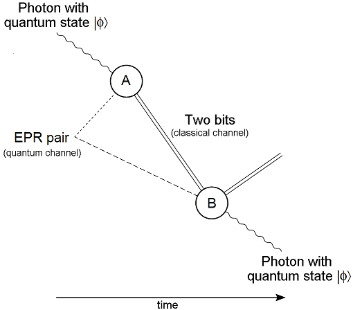
Diagram above is for quantum teleportation of a photon

Teleportation is the transfer of a quantum state from one place to another through classical channels. That teleportation is possible is surprising since quantum mechanics tells us that it is not possible to clone quantum states or even measure them without disturbing the state. Thus, it is not obvious what information could be sent through classical channels that could possibly enable the reconstruction of an unknown quantum state at the other end. Dense coding, a dual to teleportation, uses a single quantum bit to transmit two bits of classical information. Both teleportation and dense coding rely on the entangled states described in the EPR experiment. Two applications combining quantum gates and entangled states are teleportation and dense coding.

Quantum teleportation works by creating pairs of entangled photons and then sending one of each pair to the sender of data and the other to a recipient. When Alice receives her entangled photon, she lets it interact with a “memory qubit” that holds the data she wants to transmit to Bob. This interaction changes the state of her photon, and because it is entangled with Bob’s, the interaction instantaneously changes the state of his photon too. In effect, this “teleports” the data in Alice’s memory qubit from her photon to Bob’s.

The graphic below lays out the process in a little more detail:

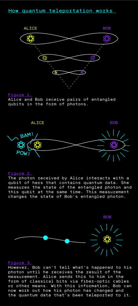
Researchers in the US, China, and Europe are racing to create teleportation networks capable of distributing entangled photons. But getting them to scale will be a massive scientific and engineering challenge. The many hurdles include finding reliable ways of churning out lots of linked photons on demand, and maintaining their entanglement over very long distances—something that quantum repeaters would make easier.

Still, these challenges haven’t stopped researchers from dreaming of a future quantum internet.

__

Charles H Bennet with his group and Stephen Wiesner have suggested a remarkable procedure for teleporting quantum states using EPR states (entangled states) as seen in the figure below. Quantum teleportation may be described abstractly in terms of two particles, A & B. A has in its possession an unknown state |ψ> represented as:

|ψ> = α|0> + β|1>

This is a single quantum bit (qubit)-a two level quantum system. The aim of teleportation is to transport the state |ψ> from A to B. This is achieved by employing entangled states. A & B each possess one qubit of a two-qubit entangled state;

|ψ> (|0>A |0>B) + |1>A|1>B)

The above state can be rewritten in the Bell basis (|00>±|11>)), (|01>±|10>) for the first two qubit and a conditional unitary transformation of the state |ψ> for the last one, that is

(|00>+|11>) |ψ>+(|00>-|11>) σZ|ψ> + (|01>+|10>) σX |ψ> + (|01>-|10>) (-iσY|ψ>)

Where σX, σY, σZ are Pauli matrices in the |0>, |1> basis. A measurement is performed on A’s qubits in the Bell basis. Depending on the outcomes of these measurements, B’s respective states are |ψ>, σZ |ψ>, σX |ψ>, -iσZ |ψ>

A sends the outcome of its measurement to B, who can then recover the original state |ψ> by applying the appropriate unitary transformation I, σZ, σ Y or iσY depending on A’s measurement outcome. It may be noted that quantum state transmission has not been accomplished faster than light because B must wait for A’s measurement result to arrive before he can recover the quantum state.

_____

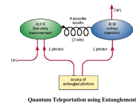
Entanglement Swapping:

Entanglement is a quantum phenomenon. When a pair of particles, such as photons, are created in a single physical process or interact with each other in a particular way, they become entangled—that is, they start behaving like a single particle, even when they become separated by any distance.

Teleportation of entanglement, also known as entanglement swapping, makes use of another curious phenomenon: It’s also possible to entangle two photons by performing a joint measurement on them, known as a Bell-state measurement. Once these photons are linked, switching the polarization of one of them—say, from up to down—causes an instantaneous switch of the other photon’s polarization, from down to up.

Here’s how the entanglement swap works: Assume you have two pairs of entangled photons, 0 and 1 in the receiving station and 2 and 3 in the transmitting station. Both entangled pairs are completely unaware of each other; in other words, no physical link exists between them. Now, assume you send photon 3 from the transmitter to the receiver and perform a Bell-state measurement simultaneously on photon 3 and on photon 1. As a result, 3 and 1 become entangled. But surprisingly, photon 2, which stayed home, is now entangled with photon 0, at the receiver. The entanglement between the two pairs has been swapped, and a quantum communication channel has been established between photons 0 and 2, although they’ve never been formally introduced.

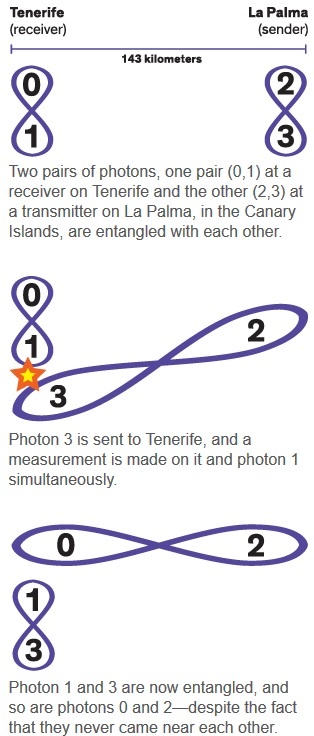
Entanglement swapping will be an important component of future secure quantum links with satellites.

The Quantum Science Satellite will be launched into a low Earth orbit and will communicate with one ground station at a time. The satellite flies over a ground station in Europe and establishes a quantum link to the ground station, and you generate a key between the satellite and the ground station in Europe. Then, some hours later, the satellite will pass a ground station in China and establish a second quantum link and secure key with a ground station in China. The satellite then has both keys available, and you can combine both keys into one key. Then you send, via a classical channel, the key combination to both of the ground stations. This you can do publicly because no one can learn anything from this combined key. Because one ground station has an individual key, it can undo this combined key and learn about the key of the other ground station.

The future quantum Internet will need a network of satellites and ground stations, similar to that of the Global Positioning System, in order to exchange quantum keys instantaneously.

______

Quantum network:

Quantum networks form an important element of quantum computing and quantum communication systems. Quantum networks facilitate the transmission of information in the form of quantum bits, also called qubits, between physically separated quantum processors. A quantum processor is a small quantum computer being able to perform quantum logic gates on a certain number of qubits. Quantum networks work in a similar way to classical networks. The main difference is that quantum networking like quantum computing is better at solving certain problems, such as modeling quantum systems.

Quantum networks for computation:

Networked quantum computing or distributed quantum computing works by linking multiple quantum processors through a quantum network by sending qubits in-between them. Doing this creates a quantum computing cluster and therefore creates more computing potential. Less powerful computers can be linked in this way to create one more powerful processor. This is analogous to connecting several classical computers to form a computer cluster in classical computing. Like classical computing this system is scale-able by adding more and more quantum computers to the network. Currently quantum processors are only separated by short distances.

Quantum networks for communication:

In the realm of quantum communication, one wants to send qubits from one quantum processor to another over long distances. This way local quantum networks can be intra connected into a quantum internet. A quantum internet supports many applications, which derive their power from the fact that by creating quantum entangled qubits, information can be transmitted between the remote quantum processors. Most applications of a quantum internet require only very modest quantum processors. For most quantum internet protocols, such as quantum key distribution in quantum cryptography, it is sufficient if these processors are capable of preparing and measuring only a single qubit at a time. This is in contrast to quantum computing where interesting applications can only be realized if the (combined) quantum processors can easily simulate more qubits than a classical computer (around 60). Quantum internet applications require only small quantum processors, often just a single qubit, because quantum entanglement can already be realized between just two qubits. A simulation of an entangled quantum system on a classical computer cannot simultaneously provide the same security and speed.

_

Overview of the elements of a quantum network:

The basic structure of a quantum network and more generally a quantum internet is analogous to a classical network.

First, we have end nodes on which applications are ultimately run. These end nodes are quantum processors of at least one qubit. Some applications of a quantum internet require quantum processors of several qubits as well as a quantum memory at the end nodes.

Second, to transport qubits from one node to another, we need communication lines. For the purpose of quantum communication, standard telecom fibers can be used. Over long distances, the primary method of operating quantum networks is to use optical networks and photon-based qubits. This is due to optical networks having a reduced chance of decoherence. Optical networks have the advantage of being able to re-use existing optical fiber. Alternately, free space networks can be implemented that transmit quantum information through the atmosphere or through a vacuum. For networked quantum computing, in which quantum processors are linked at short distances, different wavelengths are chosen depending on the exact hardware platform of the quantum processor.

Third, to make maximum use of communication infrastructure, one requires optical switches capable of delivering qubits to the intended quantum processor. These switches need to preserve quantum coherence, which makes them more challenging to realize than standard optical switches.

Finally, one requires a quantum repeater to transport qubits over long distances. Repeaters appear in-between end nodes.  Since qubits cannot be copied, classical signal amplification is not possible. By necessity, a quantum repeater works in a fundamentally different way than a classical repeater.

____

Quantum internet:

The internet has had a revolutionary impact on our world. The vision of a quantum internet is to provide fundamentally new internet technology by enabling quantum communication between any two points on Earth. Such a quantum internet will—in synergy with the “classical” internet that we have today—connect quantum information processors in order to achieve unparalleled capabilities that are provably impossible by using only classical information.

As with any radically new technology, it is hard to predict all uses of the future quantum internet. However, several major applications have already been identified, including secure communication, clock synchronization, extending the baseline of telescopes, secure identification, achieving efficient agreement on distributed data, exponential savings in communication, quantum sensor networks, as well as secure access to remote quantum computers in the cloud.

Central to all these applications is the ability of a quantum internet to transmit quantum bits (qubits) that are fundamentally different than classical bits. Whereas classical bits can take only two values, 0 or 1, qubits can be in a superposition of being 0 and 1 at the same time. Moreover, qubits can be entangled with each other, leading to correlations over large distances that are much stronger than is possible with classical information. Qubits also cannot be copied, and any attempt to do so can be detected. This feature makes qubits well suited for security applications but at the same time makes the transmission of qubits require radically new concepts and technology. Rapid experimental progress in recent years has brought first rudimentary quantum networks within reach, highlighting the timeliness and need for a unified framework for quantum internet researchers. Although a full-blown quantum internet, with functional quantum computers as nodes connected through quantum communication channels, is still some ways away, the first long-range quantum networks are already being planned.

Wehner et al propose stages of development toward a full-blown quantum internet and highlight experimental and theoretical progress needed to attain them.  Each stage is characterized by an increase in functionality at the expense of greater technological difficulty. Wehner et al. review provides a clear definition of each stage, including benchmarks and examples of known applications, and provides an overview of the technological progress required to attain these stages as seen in the figure below.

____

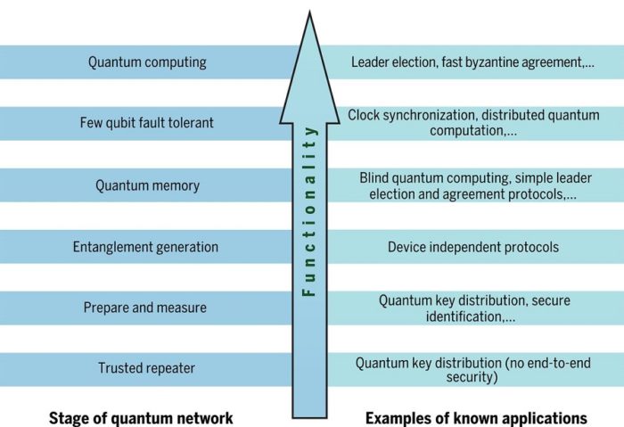
Quantum internet closer using entanglement:

Physicists in China have forged a mysterious quantum connection between particles, called entanglement, over dozens of kilometers of standard optical fiber, setting a new record. The advance marks a long step toward a fully quantum mechanical internet—although such a network is still years away. Entanglement links the strange states of tiny quantum mechanical objects. For example, a top can spin either clockwise or counterclockwise, but an atom can spin both ways at once—at least until it is measured and that two-way state collapses one way or the other. Two atoms can be entangled so that each is in an uncertain two-way state, but their spins are definitely correlated, say, in opposite directions. So if physicists measure the first atom and find it spinning clockwise, they know instantly the other one must be spinning counterclockwise, no matter how far away it is. Entanglement would be key to a fully quantum internet that would let quantum computers of the future communicate with one another and be immune to hacking.

The basic idea of the experiment is relatively simple. Researchers start with two identical stations in a single lab, each containing a cloud of rubidium atoms. Prodding each cloud with a laser, they generate a photon whose polarization, which can corkscrew clockwise or counterclockwise, is entangled with the cloud’s internal state. They then send the photons down two parallel optical fibers to a third station in another lab 11 kilometers away, where the photons interact in a way that instantly passes the original entanglement connection to the two faraway atom clouds.

To do that, physicists take advantage of the fact that, according to quantum mechanics, a measurement can affect the state of the measured object. At the destination lab, the physicists set up a measurement of the photons’ polarizations that, even as it consumes the photons, it also “projects” them into a specific entangled state with 25% probability. For those trials, the measurement instantly passes the entanglement back to the atom clouds. The researchers performed a variant of the experiment that extended the link from 22 kilometers to 50 kilometers, albeit with fibers wound on spools.

To make the experiment work, the team had to get several elements just right. A major hurdle was avoiding absorption of the photons in the optical fiber. To do that, Pan and colleagues used another laser pulse and a device called a waveguide to stretch the photons’ wavelength 60% to the sweet spot for transmission down a standard optical fiber. At the same, the researchers made life easier for themselves because the atoms clouds were actually less than 1 meter apart and merely connected by a long optical fiber. That closeness made synchronizing the experiment significantly simpler. So, strictly speaking, the record of entangling atomic-scale particles separated by 1.3 kilometers still stands, says, Ronald Hanson, a physicist at Delft University of Technology, who led that earlier effort.

Still, the experiment is significant because, for a network, the setup link is about half of the basic element called a quantum repeater. A repeater would consist of two systems like the one in the experiment placed end to end. Once physicists had entangled the atom clouds at the ends of each system, they could perform additional measurements on clouds in the middle that would swap the entanglement to the clouds on the ends, stretching the entanglement twice as far. This experiment is a big step toward a quantum repeater. But several aspects of the work need to be improved before it can be used to make a quantum repeater. In particular, the atom clouds do not yet hold their delicate quantum states long enough to allow the multiple linking needed in a quantum repeater. Pan agrees, but says his group is working on that and urges patience. “I think a true quantum network is at least 10 years away.”

_____

Scientists from Argonne and the University of Chicago entangled photons across a 52-mile network, an important step in developing a national quantum internet, a 2020 study:

Scientists from Argonne National Laboratory and the University of Chicago entangled photons across a 52-mile network in the Chicago suburbs, an important step in developing a national quantum internet. The quantum loop, spearheaded by Chicago professor and Argonne senior scientist David Awschalom, ran its first successful entanglement experiments on Feb. 11, 2020. Headquartered at Argonne, the loop is among the longest land-based quantum networks in the nation.

The experiment, funded by the U.S. Department of Energy’s Office of Science Basic Energy Sciences, is seen as a foundational building block in the development of a quantum internet— potentially a highly secure and far-reaching network of quantum computers and other quantum devices.

In the subatomic quantum world, particles can become entangled, sharing their states even though they’re in different locations—a phenomenon which could be used to transfer information. The network, which originates at Argonne in Lemont, Ill. and winds circuitously in a pair of 26-mile loops through several of Chicago’s western suburbs, taps the unique properties of quantum mechanics to eventually “teleport” information virtually instantaneously across a distance. As a bonus, scientists believe the information would be extremely difficult to hack: Quantum states change when observed, so the presence of an outside listener would actually change the signal itself.

Though quantum technology holds a great deal of promise, it’s mostly theoretical right now; quantum systems are extremely sensitive to interference and to date have been mainly tested in clean, controlled lab environments. This experiment instead runs through an existing underground network of optical fiber, built decades ago for conventional telecommunications. In the real world, the fiber cables are expanding and contracting as the temperature changes. There is also vibration and noise from the environment such as local traffics. These are all factors that can affect the quantum signal transmission, and that we can only find out by performing an experiment of this magnitude under real-world operating conditions. Many tests of quantum technologies are confined to a research environment. One of the exciting aspects of this project is the expansion of laboratory into the greater Chicago area.

_____

Diamond and quantum internet:

Creating well-functioning qubits is only one aspect of quantum computing. An equally important goal is the creation of a quantum information network — a quantum internet — that will be more secure than today’s internet. Nathalie de Leon, assistant professor of electrical engineering, is testing the viability of synthetic diamonds as devices that store and transmit information from one place to the next. Although a diamond may look clear and flawless, a close examination reveals something very different. “If you take a diamond and pull it out of the ground and look at it, you’ll notice all these little defects,” de Leon said. These defects give diamonds their color, but it turns out that they also can store and transmit information. De Leon and her colleagues figured out that by replacing two carbon atoms with a silicon atom, this particular flaw in diamonds can act as a perfect receptacle to catch a photon. Photons already carry information via the optical fibers of today’s internet, and they can also be used to carry quantum information. De Leon and her team are working to transmit quantum information from photons to electron spins, where further fine-tuning can prolong the quantum state by keeping electron spins in the proper orientation. Quantum entanglement ensures that this new kind of internet is secure against hackers. Any attempt to eavesdrop on the transmission will perturb its state. By comparing the transmitted photon to its entangled twin, the receiver can tell if an eavesdropper has disrupted the transmission. “As long as the laws of physics are correct, our channel is secure,” de Leon said.

_____

Current status of Networking in the quantum world:

True quantum networking would allow qubits to flow seamlessly across the network and to support entanglement between distant quantum machines. Clearly, we are not there yet, and not even close. Lots of research is needed. At present, there is no network connecting quantum processors, or quantum repeaters deployed outside a lab.

______

______

Moral of the story:

_

1. All ways of expressing information (i.e. voice, video, text, data) use physical system, for example, spoken words are conveyed by air pressure fluctuations. Information cannot exist without physical representation. Information, the 1’s and 0’s of classical computers, must inevitably be recorded by some physical system – be it paper or silicon. The basic idea of classical (conventional) computing is to store and process information.

_

2. Due to quantum mechanics, we were able to build devices whose functionalities extended beyond the capabilities of classical physics: computer and internet, lasers, digital cameras, MRI scanners etc. These devices are often referred to belonging to the first quantum revolution i.e. quantum 1.0

Quantum technologies are often described as the second quantum revolution i.e. quantum 2.0. These are generally regarded as a class of device that actively create, manipulate and read out quantum states of matter, often using the quantum effects of superposition and entanglement. Quantum 2.0 is expected to be highly disruptive in three major domains: communication, measurement & sensing, and computation.

_

3. Quantum computing merges two great scientific revolutions of the 20th century: quantum physics and computer science. It is the physical limitations of the classical computer and the possibilities for the quantum computer to perform certain useful tasks more rapidly than any classical computer, which drive the study of quantum computing. Quantum computation is the field that investigates the computational power and other properties of computers based on quantum-mechanical principles. An important objective is to find quantum algorithms that are significantly faster than any classical algorithm solving the same problem. Quantum physics is the theoretical basis of the transistor, the laser, and other technologies which enabled the computing revolution. But on the algorithmic level, today’s computing machinery still operates on ‘classical’ Boolean logic. Quantum computing is the design of hardware and software that replaces Boolean logic by quantum law at the algorithmic level i.e. using superposition and entanglement to process information.

_

4. Linear algebra is a continuous form of mathematics and is applied throughout science and engineering because it allows you to model natural phenomena and to compute them efficiently. Linear algebra is the mathematics of data and data is represented by linear equations, which are presented in the form of matrices and vectors. Classical computers are good at performing linear algebra calculations on vectors and matrices. The mathematical structure of quantum mechanics is based in large part on linear algebra. Quantum computation inherited linear algebra from quantum mechanics as the supporting language for describing this area. Therefore, it is essential to have a solid knowledge of linear algebra to understand quantum computation and quantum algorithms. Quantum mechanics, which is the underlying foundation for quantum computing, is heavily based on the use of linear algebra for describing quantum states in terms of wave functions as linear combinations of basis states with probability amplitudes, such that the sum of the probabilities for all states is exactly 1.0 by definition.

_

5. The use of transistors in computers is binary: if the electricity flows through the transistor, the bit, or binary digit, is 1; and if the current does not flow, the bit is 0. Whether a switch is on or off generates the ones and zeros that underlie all computer code. This is what Alan Turing discovered in his pioneering work: Simple rules for turning those switches on and off can be used to solve any mathematical problem. A computer encodes information in a series of bits, and performs operations on them using circuits called logic gates which are made from a number of transistors connected together. Logic gates simply apply a given rule to a bit. An algorithm is a well-defined procedure, with finite description, for realizing an information-processing task. In physical terms, the algorithm that performs a particular calculation takes the form of an electronic circuit made from a number of logic gates, with the output from one gate feeding in as the input to the next. Engineers can design circuits which perform addition, subtraction, multiplications… almost any operation that comes to mind, as long as the input and output information can be encoded in bits. So at their core, all digital computers have something in common. They all perform simple arithmetic operations. Their power comes from the immense speed at which they are able to do this. A classical processor performs one operation in a nanosecond i.e. billion operations per second. Operations are performed sequentially one after another but it is so fast that it appears simultaneously. Remember classical rules determine the properties of conventional logic gates in circuits. Traditional computing devices adhere to the laws of classical mechanics and are thus referred to as ‘classical computers.’

_

6. The number of transistors per inch on integrated circuit will double every 2 years. This prediction was formulated by Gordon Moore in 1965. With transistors, the name of the game is miniaturization. The smaller the transistor, the more of them it is possible to compress into the silicon slice, and the more complex are the calculations one can perform. A dual-core mobile variant of the Intel Core i3/i5/i7 has around 1.75 billion transistors for a die size of 101.83 mm². This works out at a density of 17.185 million transistors per square millimeter. Moreover, a larger number of transistors means that a given computer system could be able to do more tasks rapidly. As a consequence of the relentless, Moore’s law-driven miniaturization of silicon devices, it is now possible to make transistors that are only few tens of atoms long. At this scale, however, quantum physics effects begin to prevent transistors from performing reliably – a phenomenon that limits prospects for future progress in conventional computing and end to Moore’s law. The problem will arise when the new technologies allow to manufacture chips with around 5 nm size transistor. When it comes down to the nanometer size, electrons escape from the channels where they circulate through the so-called “tunnel effect”, a typically quantum phenomenon. Electrons are quantum particles and they have wave-like behavior, hence, there is a possibility that a part of such electrons can pass through the walls between which they are confined. Under these conditions the chip stops working properly. Tiny matter obeys the rules of quantum mechanics, which are quite different from the classical rules that determine the properties of conventional logic gates. The process of miniaturization that has made current classical computers so powerful and cheap, has already reached micro-levels where quantum effects occur. Chip-makers tend to go to great lengths to suppress these quantum effects. Transistors are just about as small as we can make them: we’re getting to the point where the laws of physics seem likely to put a stop to Moore’s Law. With the size of components in classical computers shrinking to where the behaviour of the components is practically dominated by quantum theory than classical theory, we have to explore the potential of these quantum behaviours for computation. So quantum computing is the next logical step to the physical limits of classical computing.

_

7. Newtonian world breaks down at the subatomic level. In the quantum world, everything seems to be an ocean of interconnected possibilities. Both photons and electrons show wave-particle duality and are described using the same mathematical function, the wave function. Every particle is just a wave function and could be anywhere at any time; it could even be at several places simultaneously. They are particles, in the sense that they come in discrete units with definite, reproducible properties. But the quantum-mechanical sort of “particle” cannot be associated with a definite location in space. Instead, the possible results of measuring its position are given by a probability distribution. And that distribution is given as the square of a space-filling field, its so-called wave function. Where a particle shows up is related to the square of the absolute value of the probability amplitude of its wave function. The wave function provides information about the probability amplitude of energy, momentum, and other physical properties of a particle. The wave function is what enables superposition and even entanglement. Wave function collapse means that a measurement has forced or converted a quantum (probabilistic) state into a definite measured value.

The uncertainty principle of quantum mechanics means that the more closely one pins down one measurement (such as the position of a particle), the less accurate another complementary measurement pertaining to the same particle (such as its speed) must become. Because of the uncertainty principle, statements about both the position and momentum of particles can only assign a probability that the position or momentum will have some numerical value. A probability distribution assigns probabilities to all possible values of position and momentum.

_

8. Quantum bits (qubits) are the basic unit of data in quantum computing. Qubit is the basic unit of quantum information — the quantum version of the classical binary bit physically realized with a two-state device. Qubit is a two-level quantum-mechanical system. Physically, qubits can be any two-level system. For example, the polarization of a photon (Horizontal or Vertical), or the spin of an electron (Upward or Downward). Where a bit can store either a zero or a one, a qubit can store a zero, a one, both zero and one, or an infinite number of values in between—and be in multiple states (store multiple values) at the same time! In a normal computer, a bit can be in two states — off or on. Zero or one. With the qubit, those two states aren’t the only ones possible. That’s because the spin state of an electron is described by a quantum-mechanical wave function. And that function involves two complex numbers, α and β (called quantum amplitudes), which, being complex numbers, have real parts and imaginary parts. So qubit can be in many states at once. That means a single qubit can contain exponentially more information than a normal bit. If you add more bits to a regular computer, it can still only deal with one state at a time. But as you add qubits, the power of your quantum computer grows exponentially. Physical realization of a qubit can be any small particle that due to its tiny size exhibits quantum properties, for example an atom, a photon, an electron, an ion, or any quantum system that can have two states. Devices that perform quantum information processing are known as quantum computers. Currently, the largest quantum computers (based on superconducting qubits or ion-trap qubits) have a few dozen qubits.

_

9. A bit (short for binary digit) is the smallest unit of data in a computer. A bit has a single binary value, either 0 or 1. All calculations are done using these two values (0 and1) and all calculations are done sequentially one after another. In quantum computing there is qubit having value of 1 or 0 or both or all values between 0 and 1. Even single qubit enables interesting application like secure key distribution, and more complex calculations require more qubits, and all calculations are done simultaneously in one operation only no matter number of input variables. As number of qubits increases, the computing power increases exponentially. In classical computing as the number of transistors increases, the computing power increases linearly and not exponentially. Bits are on or off voltage/current in transistor but qubit is mathematical wave function of electron spin or photon polarization.

_

10. Quantum computing is the use of quantum-mechanical phenomena such as superposition and entanglement to perform computation. Quantum computers rely on the physical properties of electrons, photons, and other tiny bits of matter that are subject to the laws of quantum mechanics. This kind of tiny matter is best described in states called amplitudes (like waves, since the tiniest bits of matter can act as both particles and waves). The basis of quantum computing is quantum wave function which is a mathematical formulation of the states of a quantum system. It represents the complete state of the quantum computer, in terms of probabilities for each of the quantum states. Wave function is variable quantity that mathematically describes the wave characteristics of a particle. The wave function is what enables superposition and entanglement. The wave function’s symbol is the Greek letter psi ψ. The wave function ψ is a mathematical expression. There is a separate wave function for each qubit or pair of entangled qubits. The individual states of a quantum system are known as basis states or basis vectors. For qubits there are two basis states — |0> and |1> which are actual states of the underlying quantum system, the physical qubit. As an example |0⟩ could represent the spin-down state of an electron while |1⟩ could represent the spin-up state. But actually the electron can be in a linear superposition of those two states i.e. |ψ⟩ electron = α∣0⟩+β∣1⟩ where α and β are complex number in such way that α² + β² = 1. A particle can have two different amplitudes (α and β) at the same time — a state called superposition. They can also be entangled, meaning a change in one particle instantly changes another. The amplitudes of particles can also cancel one another out like opposing waves in water would. Also, the smallest particles in nature don’t really exist in a point in space but they exist as a probability of existing.

You cannot examine the wave function of a quantum system (each qubit or pair of entangled qubits) without causing it to collapse. Collapse of the wave function is not a complete loss, since it collapses into a specific value of 0 or 1 for each qubit which you attempt to observe or measure, but you do lose the probability values (called probability amplitudes) for each of the superimposed and entangled quantum states of the qubit. To solve this problem, one can use quantum interference and quantum entanglement for measurement.

_

11. Quantum bits (qubit) are made of tiny particles, namely individual photons or electrons or atoms. Because these tiny particles conform more to the rules of quantum mechanics than classical mechanics, they exhibit the bizarre properties of quantum particles. Qubits can be in a 1 or 0 quantum state. But they can also be in a superposition of the 1 and 0 states. A qubit only ‘chooses’ one state or the other – at random, though the probability depends on how much up and down are in the superposition – when it is measured. Until then qubits inside a quantum computer can effectively perform multiple calculations simultaneously. Quantum computational power is determined by how many qubits a machine can simultaneously leverage. While a conventional computer with N bits at any given moment must be in one of its 2^N possible states, the state of a quantum computer with N qubits is described by the values of the 2^N quantum amplitudes, which are continuous parameters (ones that can take on any value, not just a 0 or a 1). So a quantum computer with N qubits would be in 2^N states simultaneously. This is the origin of the supposed power of the quantum computer, but it is also the reason for its great fragility and vulnerability. A quantum computer with N qubits can represent and operate on 2^N distinct and superimposed quantum states, all at the same time –that a two-qubit machine allows for four calculations simultaneously, a three-qubit machine allows for eight calculations, and a four-qubit machine performs 16 simultaneous calculations.

In the same time it takes to compute the output for a single input state on a classical computer, a quantum computer can compute the values for all input states. This process is known as quantum parallelism. Quantum mechanics describes systems in terms of superpositions that allow multiple distinguishable inputs to be processed simultaneously, though only one can be observed at the end of processing, and the outcome is generally probabilistic in nature. The superposition of qubits is what gives quantum computers their inherent parallelism and this parallelism allows a quantum computer to work on a million computations at once, while your desktop PC works on one. A 30-qubit quantum computer would equal the processing power of a conventional computer that could run at 10 teraflops (trillions of floating-point operations per second). Today’s typical desktop computers run at speeds measured in gigaflops (billions of floating-point operations per second).

_

12. Entanglement is a quantum phenomenon. When a pair of particles, such as photons, are created in a single physical process or interact with each other in a particular way, they become entangled—that is, they start behaving like a single particle, even when they become separated by any distance. When one entangled particle is measured – and hence ‘chooses’ a state – its partner is immediately bound by that choice, no matter how far away it is. In an entangled system, two seemingly separate particles can behave as an inseparable whole. Theoretically, if one separates the two entangled particles, one would find that their velocity of spin would be identical but in opposite directions. When measurement of any two-valued state of a particle (such as light polarized up or down) is made on either of two ‘entangled’ particles that are very far apart, it causes a subsequent measurement on the other particle to always be the other of the two values (such as polarized in the opposite direction).

Entanglement is useful in quantum measurement, scalability, increasing complexity, speed-ups and quantum communications. When the two particles are entangled, the change in state of one particle will alter the state of its partner in a predictable way, which comes in handy when it comes time to get a quantum computer to calculate the answer to the problem you feed it. Entanglement allows scientists to know the value of the qubits without actually looking at them. Quantum entanglement play an important role in the observed computational speed-up of some quantum algorithms. It is proved that entanglement is involved in quantum algorithms, such as Grover’s and Shor’s algorithms.

Realizing the potential for scalability of quantum computers is a major challenge, and in many cases not even achievable, at least in the relatively near future. Connectivity of qubits is likely to be a real issue. Or rather the significant restrictions on connectivity on current quantum computers is an issue. Qubit connectivity means any 2 qubits can be connected (entangled) to perform 2-qubit operations. Connectivity may not grow at the same rate as qubit count grows. When trying to predict the future progress of quantum computers, the qubit count is often used as the primary indicator. This is misleading as there are other parameters that can inhibit the progress of quantum computers, even when the qubit count continues to increase. Connectivity may not grow at the same rate as qubit count grows. Entanglement isn’t easy to implement in hardware. And even when connectivity does increase, it doesn’t keep up with the raw number of quantum states which those qubits support. A 10-qubit quantum computer supports 2¹⁰ (1024) quantum states, but only five concurrent entangled pairs of qubits, and not all combinations of pairs. A 20-qubit quantum computer supports a million quantum states, but only ten concurrent entangled pairs of qubits, and not all combinations of pairs. So, algorithms must use entanglement very sparingly, which limits scalability. This significantly reduces the ability to run complex quantum algorithms. Shor’s algorithm was billed as killing public-key encryption, but once again, an algorithm which works very well with a small amount of data simply doesn’t scale. The better the connectivity of a device, the faster and easier it will be for us to implement powerful quantum algorithms.

_

13. Quantum logic gates are instructions (software), unlike classical logic gates which are hardware. Quantum gates transform the state of qubits. Quantum logic circuits are instruction sequences, not electronic circuits. A quantum circuit is composed by qubits and gates operating on those qubits. All quantum gates are of reversible nature as all quantum gates are unitary matrices. A unitary matrix is any square matrix of complex numbers such that the conjugate transpose is equal to its inverse. One general feature of quantum gates that distinguishes them from classical gates is that they are always reversible: the inverse of a unitary matrix is also a unitary matrix, and thus a quantum gate can always be inverted by another quantum gate. Quantum gates are represented by matrices, and can be visualised as rotations over the Bloch sphere.

_

14. A classical (or non-quantum) algorithm is a finite sequence of instructions, or a step-by-step procedure for solving a problem, where each step or instruction can be performed on a classical computer. Similarly, a quantum algorithm is a step-by-step procedure, where each of the steps can be performed on a quantum computer. Although all classical algorithms can also be performed on a quantum computer, the term quantum algorithm is usually used for those algorithms which seem inherently quantum, or use some essential feature of quantum computation such as quantum superposition or quantum entanglement. Quantum computers are capable of performing any computation which a classical deterministic computer can do.

Problems which are undecidable using classical computers remain undecidable using quantum computers. What makes quantum algorithms interesting is that they might be able to solve some problems faster than classical algorithms because quantum superposition and quantum entanglement that quantum algorithms exploit probably can’t be efficiently simulated on classical computers. An important parameter to the success of a quantum algorithm is its performance compared to classical algorithms. From a theoretical point of view there are certain computational problems that are proven to be intractable with classical computers (or at least infeasible within a reasonable time). An implementation of a quantum algorithm that solves such a problem would be a great achievement.

Shor’s algorithm is used for factorization of large numbers and solving the discrete logarithm problem. This algorithm has the potential to break most of the currently used public-key cryptography.

Grover’s algorithm is used for searching in an unsorted list. This is a generic method that can be applied to many types of computational problems. The running time of Grover’s algorithm on a quantum computer will scale as the square root of the number of inputs (or elements in the database), as opposed to the linear scaling of classical algorithms.

_

15. The quantum state of any system – whether it be a qubit or some other system – is not directly observable.

We have a qubit (a superposed quantum state) formed by some linear combination of |0> and |1>.

After measurement, it becomes a classical bit (0 or 1).

Measurements destroy the quantum state in most cases as energy enters and leaves the system.

Suppose a qubit is in the state |ψ⟩ = α∣0⟩+β∣1⟩. When you measure this qubit in the computational basis it gives you a classical bit of information: it gives you the outcome 0 with probability α², and the outcome 1 with probability β².

Remember α² + β² = 1

In contrast to a classical bit, which can only be in one of its two basic states, a qubit can be in any of a continuum of possible states, as defined by the values of the quantum amplitudes α and β. This is superposition. These complex numbers, α and β, each have a certain magnitude, and according to the rules of quantum mechanics, their squared magnitudes must add up to 1. That’s because those two squared magnitudes correspond to the probabilities for the spin of the electron to be in the basic states ↑ and ↓ when you measure it. And because those are the only outcomes possible, the two associated probabilities must add up to 1. For example, if the probability of finding the electron in the ↑ state is 0.6 (60 percent), then the probability of finding it in the ↓ state must be 0.4 (40 percent)—nothing else would make sense.

A key point to note is that after the measurement, no matter what the outcome, complex numbers α and β are gone and so you can’t get any more information about them. A complex number is a number that can be expressed in the form a + bi, where a and b are real numbers, and i is a solution of the equation x² = −1. Because no real number satisfies this equation, i is called an imaginary number.

The corresponding state of the qubit after the measurement is ∣0⟩| or ∣1⟩. Basic state |0> has α = 1 and β = 0 and basic state |1> has α = 0 and β = 1

_

16. One of the great qualities of a classical computer, based on the concept of a Turing machine, is that it is strictly deterministic. Quantum computers on the other hand are inherently probabilistic rather than deterministic, just as with the quantum mechanics upon which quantum computing is based. Rather than calculating the answer to a problem as a classical computation would do, a quantum computation generates the probabilities for any number of possible solutions. While a quantum system can perform massive parallel computation, access to the results of the computation is restricted. Accessing the results is equivalent to making a measurement, which disturbs the quantum state. We can only read the result of one parallel thread, and because measurement is probabilistic, we cannot even choose which one we get.

_

17. For computers to function properly, they must correct all small random errors. In a quantum computer, such errors arise from the non-ideal circuit elements and the interaction of the qubits with the environment around them. For these reasons the qubits can lose coherency in a fraction of a second and, therefore, the computation must be completed in even less time. If random errors – which are inevitable in any physical system – are not corrected, the computer’s results will be worthless. These errors cause the ideal shape of the Bloch Sphere to deform in different ways based on the channels of error (i.e. bit flips, phase flips, depolarizing, amplitude dampening, or phase dampening) and their rate. In order to achieve suitable quantum error correction an architecture may have to expend multiple physical qubits to construct a resulting single functioning logical qubit. As a computation begins, the initial set of qubits in the quantum computer are referred to as physical qubits. Error correction works by grouping many of these fragile physical qubits, which creates a smaller number of usable qubits that can remain immune to noise long enough to complete the computation. These stronger, more stable qubits used in the computation are referred to as logical qubits. The ratio of physical qubit to logical qubit is very large for error correction in quantum computation. At a 0.1% probability of a depolarizing error, the surface code would require approximately 1,000-10,000 physical qubits per logical qubit. Therefore so-called “universal” quantum computer is further off. The reason is errors, lots of them. Scientists have only been able to keep qubits in a quantum state for fractions of a second — in many cases, too short a period of time to run an entire algorithm. And as qubits fall out of a quantum state, errors creep into their calculations. These have to be corrected with the addition of yet more qubits, but this can consume so much computing power that it negates the advantage of using a quantum computer in the first place. Balancing fidelity of the system with scalability is needed. The larger the scale (that is, number of qubits), the higher the error rate. Not only do programs need to be constrained, but they need to be run many times, as current qubit implementations have a high error rate. To get the right answer from a quantum computer, researchers either have to repeat a calculation an unreasonable number of times, or build a quantum computer with millions of qubits.

_

18. The state of superposition, which is necessary to perform calculations, is difficult to achieve and enormously hard to maintain. Physicists use laser and microwave beams to put qubits in this working state and then employ an array of techniques to preserve it from the slightest temperature fluctuations, noises and electromagnetic waves. If a stray photon — a particle of light — from outside the system were to interact with a qubit, its wave would interfere with the qubit’s superposition, essentially turning the calculations into a jumbled mess – a process called decoherence. As long as there exists a definite phase relation between different states, the system is said to be coherent. A definite phase relationship is necessary to perform quantum computing on quantum information encoded in quantum states. Quantum computers are extremely sensitive to interaction with the surroundings since any interaction (or measurement) leads to a collapse of the state function. This phenomenon is called decoherence. It is extremely difficult to isolate a quantum system, especially an engineered one for a computation, without it getting entangled with the environment. The larger the number of qubits the harder is it to maintain the coherence. One of the greatest challenges is controlling or removing quantum decoherence. This usually means isolating the system from its environment as interactions with the external world cause the system to decohere. However, other sources of decoherence also exist. Examples include the quantum gates, and the lattice vibrations and background thermonuclear spin of the physical system used to implement the qubits. Decoherence is irreversible, as it is effectively non-unitary, and is usually something that should be highly controlled, if not avoided.

When a quantum computer is operating, it needs to be placed in a large refrigerator to cool the device to less than a degree above absolute zero. This is done to keep energy from the surrounding environment from entering the machine. Qubits must be shielded from all external noise, since the slightest interference will destroy the superposition, resulting in calculation errors. Well-isolated qubits heat up quickly, so keeping them cool is a challenge. The current operating temperature of quantum computers is 0.015 Kelvin or -273C or -460F. That is the only way to slow down the movement of atoms, so a “qubit” can hold a value. Qubits must be kept cold enough to maintain an entangled superposition of states. Even at such a low temperature, qubits are only stable (retaining coherence) for a very short time. This greatly limits the flexibility of programmers in how many operations they can perform before needing to read out a result. The quantum state will tend to decay within a very tiny fraction of a second — less than one 10,000th of a second, 90 microseconds, on the 50-qubit IBM quantum computer. Coherence time is a period during which qubits hold their quantum state. Coherence time should be longer than gate-operation time.

_

19. These are the three most important aspects of a quantum device: qubit number (correlates with number of simultaneous operations due to superposition), connectivity (correlates with entanglement and its benefits) and noise level (correlates with erroneous calculations). To have any idea of what a quantum computer can do, you need to know them all.

_

20. In a general structure of a quantum computer system, the user interacts with a classical computer. For example, if the problem requires optimization, the classical computer translates the user’s problem into a standard form for a quantum computer or into a different form if another quantum algorithm is required. Transforming real data to and from the form of data that exists on a quantum computer is performed on a classical computer. The classical computer creates control signals for qubits located in a cryogenic environment to receive data from measurements of the qubits. You are going to a quantum computer to solve certain coordinates of a problem and get the result back from the classical computer. Some classical electronics are placed in the cold environment to minimize heat flow through wiring across the cryogenic-to-room-temperature gradient.

_

21. Two key factors make quantum computers far more powerful than the most powerful supercomputer known to us today.

These are:

-1. Quantum Parallelism

A 4-bit classical computer register can hold any one of 16 (2⁴) possible numbers. In contrast, a 4-qubit quantum computer register can hold 16 different numbers simultaneously.

-2. Exponential increase in computing ability with the addition of each qubit

Each single qubit you add doubles the states the system can simultaneously store: Two qubits can store four states, three qubits can store eight states, and so on. Thus, you might need just 50 qubits to model quantum states that would require exponentially many classical bits — 1.125 quadrillion to be exact — to encode. A quantum machine could therefore make the classically intractable problem of simulating large quantum-mechanical systems tractable, or so it appears. This gives quantum computers processing power that is beyond the scope of a classical computer.

_

22. In mathematics and computer science, an optimization problem is the problem of finding the best solution from all feasible solutions. An optimization problem is essentially finding the best solution to a problem from endless number of possibilities. Classical computers would have to configure and sort through every possible solution one at a time, on a large-scale problem this could take millions of years. Quantum computers can find all possible variants at the same time using superposition and entanglement and sift through large amounts of input varables in a significantly small amount of time. Applications range from transportation and logistics, healthcare, software design, finance, web search, genomics, diagnostics, and material science.

_

23. Computational complexity theory is a way of categorizing various styles of computer problems into classes based on how hard it is for a computer to solve them. The class of problems that quantum computers can solve efficiently is called BQP which cannot be solved by classical computers in polynomial time. Quantum computers cannot efficiently solve NP-complete problems in polynomial time.

_

24. Adiabatic quantum computation (AQC) is an alternative to the better-known gate model of quantum computation. The two models are polynomially equivalent, but otherwise quite dissimilar: one property that distinguishes AQC from the gate model is its analog nature. Quantum annealing (QA) describes a type of heuristic search algorithm that can be implemented to run in the native instruction set of an AQC platform. The first difference your bound to notice between relatively conventional quantum computers and quantum annealing computers is the number of qubits they use. While the state-of-the-art in conventional quantum computers is pushing a few dozen qubits in 2019, the leading quantum annealer has more than 2000 qubits. Of course, the trade-off is that quantum annealers are not universal but specialized quantum computers that technically tackle only optimization problems and sampling problems. Universal quantum computers are based on logical gates and work similar to the underlying logic foundations of classical computers. Universal quantum computers are the most powerful and most generally applicable, but also the hardest to build. A truly universal quantum computer would likely make use of about 1 million qubits.

_

25. Quantum computers will never “replace” classic computers, simply because there are some problems that classic computers are better and/or more efficient at solving. Classical computers are better at some tasks than quantum computers (email, spreadsheets and desktop publishing to name a few). Quantum computers are not very good at the three R: reading, writing and arithmetic. They don’t like to read big databases, they can’t give you very big complicated readouts, and they don’t do regular arithmetic as well as a classical computer. The difficulty of attempting classic calculations on quantum computers is not widely understood, leading to optimistic predictions about their applicability for general-purpose use cases. Classical computers have large memories capable of storing huge datasets — a challenge for quantum devices that have only a small number of qubits. On the other hand, quantum algorithms perform better for certain problems than classical algorithms.

The intent of quantum computers is to be a different tool to solve different problems, not to replace classical computers. Typically, the problem set that quantum computers are good at solving involves number or data crunching with a huge amount of inputs, such as “complex optimization problems and communication systems analysis problems” — calculations that would typically take supercomputers days, years, even billions of years to brute force. Quantum computers working with classical systems have the potential to solve complex real-world problems such as simulating chemistry, modelling financial risk and optimizing supply chains. To be clear, quantum computing is expected to be designed to work alongside classical computers, not replace them.  Quantum computers are large machines that require their qubits to be kept near absolute zero (minus 273 degrees Celsius) in temperature, so don’t expect them in your smartphones or laptops. And rather than the large number of relatively simple calculations done by classical computers, quantum computers are only suited to a limited number of highly complex problems with many interacting variables.

_

26. In quantum computing, quantum supremacy is the goal of demonstrating that a programmable quantum device can solve a problem that classical computers practically cannot, but it leaves lot of questions hanging. Outperforming for which problem? How do you know the quantum computer has got the right answer if you can’t check it with a tried-and-tested classical device? And how can you be sure that the classical machine wouldn’t do better if you could find the right algorithm?

_

27. Rather than using more electricity, quantum computers will reduce power consumption anywhere from 100 up to 1000 times as compared to classical computers because quantum computers use quantum tunneling.

_

28. Potential quantum computing applications include optimization in various industries, research, cybersecurity, navigation, seismology, pharmaceuticals and healthcare, finance and banking, marketing, weather forecasting, logistics, faster data analysis, particle physics, energy usage, artificial intelligence, gene analysis, chemical synthesis, unstructured search etc.

_

29. Please differentiate between quantum simulator and quantum simulation:

Quantum simulator runs quantum algorithm on classical computer to simulate quantum mechanics on classical computer. Quantum simulation is run on quantum computer to exact computer model of a molecule or drug because quantum behaviour of electrons and atoms of such a molecule or drug is relatively close to the native behavior of a quantum computer. Photosynthesis, superconductors, and complex molecules are examples of quantum systems that can be simulated using quantum programs. Quantum simulation could also be used to simulate protein folding — one of biochemistry’s toughest problems. Misfolded proteins can cause diseases like Alzheimer’s and Parkinson’s, and researchers testing new treatments must learn which drugs cause reactions for each protein through the use of random computer modelling.

_

30. Quantum technologies may have a negative effect to cyber security, when viewed as a resource for adversaries, but can also have a positive effect, when honest parties use these technologies to their advantage.

AES-128 and RSA-2048 both provide adequate security against classical attacks, but not against quantum attacks. AES 256 and hash function SHA-256 are somewhat quantum-safe.  A 160-bit elliptic curve cryptographic key could be broken on a quantum computer using around 1000 logical qubits while factoring the security-wise equivalent 1024-bit RSA modulus would require 2000 logical qubits. And to implement Shor’s algorithm for factoring a 2048 bit number we need more than 4000 logical qubits and 20 million physical qubits. By comparison, Google’s measly 53 qubits are still no match for this kind of cryptography. Today’s quantum computers can not break current encryption schemes. To break today’s encryption requires a large-scale and fault tolerant quantum computer, and we aren’t there yet. Therefore, we’re unlikely to see a quantum computing-driven security breach in the near future. Quantum computing poses a theoretical threat to most current public-key cryptography. However, cybercriminals can siphon off data today and unlock it when quantum cryptoanalysis becomes practical. So we need quantum-resistant algorithms as soon as possible.

Post-quantum cryptography uses conventional cryptographic tools to protect from quantum computer attacks and it is distinct from quantum cryptography which refers to using quantum phenomena to achieve secrecy and detect eavesdropping. Quantum cryptography is different from traditional cryptographic systems in that it relies more on physics, rather than mathematics, as a key aspect of its security model. Essentially, quantum cryptography is based on the usage of individual particles/waves of light (photon) and their intrinsic quantum properties to develop an unbreakable cryptosystem (because it is impossible to measure the quantum state of any system without disturbing that system.)  The most well-known and developed application of quantum cryptography is quantum key distribution (QKD). QKD involves sending encrypted data as classical bits over networks, while the keys to decrypt the information are encoded and transmitted in a quantum state using qubits.  Quantum key distribution is currently used in certain situations where the need for security is high, such as banking and voting. It is still relatively expensive and cannot be used over large distances, which has prevented further adoption.

_

31. Blockchain networks including Bitcoin’s architecture relies on two algorithms: Elliptic Curve Digital Signature Algorithm (ECDSA) for digital signatures and SHA-256 as a hash function. A blockchain is secured by two major mechanisms: 1) encryption via asymmetric cryptography and 2) hashing. Powerful quantum computers could pose a serious threat to asymmetric encryption but not to hashing. They could use Shor’s Algorithm to significantly reduce the number of steps to factor big numbers, thus more easily revealing the private key associated with a given public key. They could also use Grover’s Algorithm to attempt to break cryptographic hashing more easily than a classical computer can today, but this task would still be next to impossible. However given the primitive state of quantum computing today, we cannot expect any serious challenge to blockchain security mechanisms from either of these algorithms.

_

32. Quantum Machine Learning (QML) is application of quantum computing algorithms to artificial intelligence techniques. Quantum-enhanced machine learning refers to quantum algorithms that solve tasks in machine learning, thereby improving and often expediting classical machine learning techniques. The use of quantum algorithms in artificial intelligence techniques will boost machines’ learning abilities.

_

33. Teleportation is the transfer of a quantum state (qubit) from one place to another using entanglement (pair of entangled photons) and classical communication. That teleportation is possible is surprising since quantum mechanics tells us that it is not possible to clone quantum states or even measure them without disturbing the state. True quantum networking would allow qubits to flow seamlessly across the network and to support entanglement between distant quantum machines. Clearly, we are not there yet, and not even close. Lots of research is needed.

_

34. Logistically, quantum computers are difficult to maintain and require specialized environments cooled to 0.015 Kelvin. The quantum processor must be placed in a dilution refrigerator shielded to 50,000 times less than the earth’s magnetic field and placed in a high vacuum to 10 billion times lower than atmospheric pressure. It will also need calibration several times per day. For most organizations, this is not feasible. Organizations interested in quantum computing should use quantum computing as a service (QCaaS) through the cloud.

Cloud-based quantum computing is the invocation of quantum emulators, simulators or processors through the cloud. Increasingly, cloud services are being looked on as the method for providing access to quantum processing. When users are allowed access to quantum computers through the internet it is known as quantum computing within the cloud.  Amazon Web Services (AWS) has launched Braket, a quantum computing as a service by collaborating with D-Wave, IonQ and Rigetti who will allow access to their quantum computer over internet. By 2023, 95% of organizations researching quantum computing strategies will utilize QCaaS.

_

35. Quantum computing is heavily hyped. As on today there is no commercially viable applications for near-term quantum computers that cannot already be tackled with conventional computers. Early quantum computers may not beat out conventional computers in chemistry simulations or other applications. It is not helpful when the media makes wild, speculative claims. And it’s equally unhelpful when managers, executives, and promoters help to fuel those wild, speculative efforts. Concerns about qubit connectivity, high noise levels, the effort required to correct errors, and the scalability of quantum hardware have limited ability to deliver the solutions that future quantum computing promises. There may be a limit to how many qubits can be operated on in parallel before the coherence limit is reached. Qubits are sensitive devices and prone to error. Given the nature of quantum computing, error correction is ultra-critical – even a single error in a calculation can cause the validity of the entire computation to collapse. Some researchers think that the problem of error correction will prove intractable and will prevent quantum computers from achieving the grand goals predicted for them. The only real solution is to patiently await real progress on both actual hardware and production-quality algorithms and code. In the next 10 years, expected improvements in qubits (quality, count, and connectivity), error correction, and quantum algorithms will hopefully decrease runtime and enable more advanced computation.

______

Dr. Rajiv Desai. MD.

April 12, 2020

______

Postscript:

My mathematical formula of Pi, theory of duality of existence and photon weaving theory are just drops in the ocean of science but every drop counts in science as it improves our understanding of the universe.

_____